Ensemble Learning: Bagging, Boosting, and Stacking

Ensemble methods are one of the coolest and most powerful ideas in machine learning. At their core, they're all about combining predictions from multiple models to get a better result than any single model could deliver on its own. It's the classic "wisdom of the crowd" principle, but for algorithms.

The Power of Many in Machine Learning

Think about guessing the number of jellybeans in a huge jar. If you ask one person, their guess might be wildly off. But if you ask a hundred people and average their guesses, you'll probably get remarkably close to the real number.

That’s the essence of ensemble methods in machine learning. Instead of pouring all our effort into building one perfect, all-knowing model (which is often impossible), we build a "team" of models that collaborate. Each individual model, often called a "weak learner," might have its own quirks or blind spots. But when you bring them together, their strengths start to cover for each other's weaknesses.

Why Ensembles Can Improve Generalization

So, why does this team approach work so well? It boils down to tackling the fundamental tug-of-war in machine learning: the bias-variance tradeoff. If you want a deeper dive, we cover this concept extensively in our guide to the bias-variance tradeoff.

A single, overly complex model might memorize the training data perfectly but fall apart when it sees new, real-world data. That's high variance. On the flip side, a model that's too simple might be too rigid and miss crucial patterns in the data, which is high bias.

Ensembles give us a structured way to get the best of both worlds. Here’s what you gain:

• Potential generalization benefit: Combining models can improve held-out performance when their errors are sufficiently diverse and the combination rule suits the task. It is not guaranteed.
• Rock-Solid Robustness: The final model is far less sensitive to noise or weird outliers in the training data. If one model gets thrown off by a strange data point, the others act as a correcting force, leading to much more stable and reliable predictions.
• Less Overfitting: Certain ensemble techniques, like Bagging, are specifically designed to slash variance, helping your model generalize much better to data it has never seen before.

Before we go further, here's a quick table to summarize why a team of models almost always beats a lone wolf.

Why Ensemble Methods Outperform Single Models

This table gives a quick overview of the key advantages of using ensemble techniques compared to relying on a single machine learning model.

Characteristic	Single Model Approach	Ensemble Method Approach
Error Handling	A single error can significantly skew the final prediction.	Errors from one model are often canceled out by correct predictions from others.
Overfitting Risk	Highly susceptible, especially with complex models.	Reduces overfitting by averaging out biases and variances.
Robustness	Sensitive to noise and outliers in the training data.	More resilient to outliers, as their impact is diluted across many models.
Performance	Performance is limited by the capability of one algorithm.	Achieves higher accuracy and stability by combining multiple perspectives.

Ultimately, ensembles give you a model that is not only more accurate but also more dependable in real-world scenarios.

A Practical Example: The Bank Loan Predictor

Let's make this real. Imagine a bank wants to build a model to predict if a loan applicant will default.

The Actionable Insight: The goal isn't just to predict, but to give loan officers a reliable tool to reduce financial risk. A wrong decision costs the bank real money.

A deep decision tree can fit idiosyncrasies in the training sample. A random forest averages randomized trees to reduce variance, but it does not make a lending decision fair, causal, or compliant. The bank would still need representative data, an appropriate outcome definition, subgroup and calibration analysis, policy constraints, human-review rules, and monitoring after deployment.

Now, let's try an ensemble approach, like a Random Forest. Instead of one tree, it builds hundreds, each on a slightly different slice of the data and features.

• One tree might focus heavily on age and employment history.
• Another might prioritize the applicant's debt-to-income ratio.
• A third might find a pattern in the number of open credit lines.

By polling all these "expert" trees, the bank gets a far more nuanced and trustworthy prediction. The final decision smooths out the weird biases of any single tree. When an applicant is flagged as high-risk by the ensemble, the loan officer can take concrete action, like requiring a larger down payment or offering a different loan product, directly mitigating the bank's risk exposure.

To really get what makes ensemble methods in machine learning so powerful, we need to talk about two concepts that keep every data scientist on their toes: bias and variance. Think of them as two opposing forces in a constant tug-of-war. Nailing the balance between them is the secret to building models that actually work in the real world, not just on your training data.

Let's use an analogy. Imagine you're at a carnival, throwing darts. The bullseye is your goal.

• High Bias: You throw three darts, and they all land in a tight little group in the top-left corner, way off from the bullseye. That's high bias. Your throws are consistently wrong in the same direction. It means your model has some fundamental assumption that's leading it astray. It's inaccurate but consistent.

• High Variance: You throw three more darts. One hits the top right, another the bottom left, and the third lands somewhere near the middle. On average, you’re centered around the bullseye, but your throws are all over the place. That's high variance. Your model is way too sensitive to small fluctuations, making its predictions erratic and unreliable.

The perfect thrower—like a pro dart player—has both low bias and low variance. Their darts all hit in a tight cluster right on the bullseye. Accurate and consistent. That’s the dream.

The Bias-Variance Tradeoff

Bias and variance are useful components of prediction error, but the trade-off is not a law that forces every reduction in one to increase the other. Model class, regularization, data volume, noise, and the ensemble construction all affect the balance. Evaluate the complete pipeline empirically.

A really simple model, like a basic linear regression, often has high bias because it’s just not flexible enough to capture complex relationships in the data. On the flip side, a ridiculously complex model, like a deep decision tree, can suffer from high variance. It might fit the noise in your training data so perfectly that it completely falls apart when it sees new, unseen data.

This is where ensembles come in. They give us a brilliant framework for managing this tradeoff.

Instead of hunting for one single, perfect model, ensembles build a team of models. The idea is that the members of the team can compensate for each other's flaws, attacking either high bias or high variance directly.

Defining Weak Learners

In boosting theory, a weak learner is an algorithm that can perform slightly better than chance under the assumptions of the learning problem. That formal concept is not a requirement for every ensemble: a random forest combines fully grown randomized trees, and a stacking ensemble can combine strong, heterogeneous estimators.

A classic example is a "decision stump"—a decision tree with only one or two splits. On its own, it’s not very useful. It has high bias because its rules are too simple to learn much.

But here's the magic. Ensembles have clever ways of combining these simple, error-prone models to create something incredibly strong. Their individual weaknesses are forged into a collective strength.

How Ensembles Tackle Bias and Variance

Different ensemble techniques are specifically designed to go after either bias or variance. It's this strategic approach that makes them so effective.

• Bagging for Variance Reduction: Techniques like Bagging (which we’ll get to next) are all about taming high variance. They work by training many models on different random subsets of the data and then averaging their predictions. This process smooths out the wild inconsistencies of individual models, as their errors tend to cancel each other out.

• Boosting for stage-wise loss optimization: Boosting adds learners sequentially so that the ensemble improves an objective. It often reduces bias and can also affect variance; shrinkage, tree depth, subsampling, and early stopping control overfitting.

Whether an ensemble helps depends on base-estimator quality, error correlation, combination method, regularization, and data. The following sections explain how bagging and boosting alter those factors.

Exploring Bagging and Random Forests

One of the most intuitive and powerful ensemble methods in machine learning is Bagging, which is just short for Bootstrap Aggregating. The core idea is brilliantly simple: why trust a single model when you can build a whole committee of them and let them vote? It’s a democratic process that helps smooth out any single model's weird quirks and reduces the overall variance.

The process kicks off with a technique called bootstrapping. From your original training data, you create a bunch of new, random subsets by sampling with replacement. This means some data points might show up multiple times in a subset, while others might not show up at all. The goal is to make sure each subset is just a little bit different from the others.

Once you have these bootstrapped subsets, you train a separate base model—usually a decision tree—on each one. Since every model sees a slightly different version of the data, they all learn slightly different patterns and develop their own unique perspectives. Finally, you pull all their predictions together. For classification, you take a majority vote. For regression, you average the results.

The Rise of Random Forests

The most popular and effective version of Bagging is the Random Forest algorithm. It takes the solid foundation of Bagging—training multiple decision trees on bootstrapped data—and adds another clever twist to make the models even more diverse.

In a normal decision tree, the algorithm looks at every single feature to find the best possible split at each node. A Random Forest shakes things up. At each split, it only considers a random, smaller subset of the features available. This little trick prevents one or two really strong features from dominating all the trees, forcing them to find other, more creative predictive patterns.

This double-layer of randomness—sampling data through bootstrapping and sampling features at each split—is the secret sauce behind Random Forests. It creates a collection of highly decorrelated trees whose combined prediction is way more robust and accurate than any single tree could ever be.

Bagging and boosting are distinct constructions with different assumptions and failure modes. Neither guarantees better performance than a well-selected single model, so compare them with an appropriate validation design.

Modern ensemble methods can improve generalization, but the effect size is dataset-, metric-, and validation-dependent. Report the measured difference and uncertainty for the actual task rather than a universal percentage range.

A Practical Example: Predicting Customer Churn

Let's ground this in a real-world business problem: predicting customer churn for a telecom company. Our goal is to flag customers who are likely to cancel their service. A single decision tree might get too specific and overfit the training data, creating rules based on random noise that don't hold up in the real world.

The Actionable Insight: The business needs to proactively identify at-risk customers before they leave, so the marketing team can intervene with targeted retention offers.

This is where a Random Forest shines, building hundreds of decision trees to tackle the problem.

• Tree 1 might be trained on a data subset where it learns that monthly charges and contract type are the most important features.
• Tree 2, seeing a different slice of data and a random set of features, might decide that the frequency of customer service calls and the customer's tenure are the real predictors.
• Tree 3 could zero in on a pattern involving specific add-on services and the customer's payment method.

Each of these trees is a "weak learner" with its own unique point of view. When you want to predict churn for a new customer, you run their data through the entire forest. Maybe 350 trees vote "Churn" while 150 trees vote "Stay." The final prediction is "Churn," giving the company a clear signal. This isn't just a prediction; it's a trigger for action. The marketing team can now offer that specific customer a discount, a free upgrade, or a loyalty bonus to persuade them to stay, directly impacting revenue. For a deeper dive into how this team-based approach stacks up against its core component, check out our comparison of a Random Forest vs a Decision Tree.

When Should You Use a Random Forest?

Random Forests are a fantastic go-to model for many machine learning tasks because they're so versatile and tough to break. Here’s when they are a particularly strong choice:

• When you need a strong baseline: Random Forests are easy to implement and give great results with relatively little tuning, making them a perfect starting point for almost any problem with tabular data.
• When you can define a complete preprocessing pipeline: Random-forest support for categorical and missing values varies by library and estimator. In scikit-learn, do not assume arbitrary string categories are accepted by RandomForestClassifier; preprocess features as required by the implementation, and fit preprocessing inside the validation pipeline.
• To avoid overfitting: The Bagging mechanism makes Random Forests much less likely to overfit than a single decision tree, especially with complex datasets.
• For model inspection: Tree ensembles expose impurity-based importance, but those scores can favor high-cardinality features and describe the fitted model rather than causal influence. Check predictive performance first, compute permutation importance on held-out data, and account for correlated features when interpreting either method.

If Bagging is all about teamwork through parallel, democratic effort, Boosting is more like a mentorship program. This is another powerful player in the world of ensemble methods machine learning, but it takes a completely different, sequential approach. Instead of building models that work independently, Boosting builds them one after another, where each new model is explicitly trained to fix the mistakes of the one that came before it.

Think of it like a student prepping for a tough exam. After the first try, they don't just study everything again; they zero in on the questions they got wrong. With that focused effort, their next attempt is much stronger on the tricky parts. That’s the core idea behind Boosting.

This process brilliantly transforms a series of "weak learners"—models that are just a little better than a random guess—into a single, highly accurate "strong learner." We’ll break down two of the most important boosting algorithms out there: AdaBoost, the original pioneer, and the Gradient Boosting family, with the famous XGBoost leading the pack.

AdaBoost The Original Adaptive Booster

AdaBoost, which stands for Adaptive Boosting, was one of the first algorithms to really nail this sequential learning concept. Its method is both elegant and incredibly effective. It kicks things off by training a very simple model, often just a decision stump (a one-level decision tree), on the dataset.

Once that first model makes its predictions, AdaBoost goes to work. It examines the results and increases the weight of any data points that were misclassified. In the next round, a new weak learner is trained, but this time it has to pay much closer attention to those now-heavier, harder-to-classify examples.

This cycle continues, with each new model laser-focused on the errors its predecessor made. The final prediction isn't just an average; it's a weighted vote from all the models, where the ones that performed better get a bigger say in the final outcome.

Gradient Boosting and the Power of XGBoost

Gradient boosting fits each new learner to the negative gradient of the selected loss with respect to the current ensemble prediction. For squared-error regression, those pseudo-residuals are ordinary residuals. For classification and other losses, “predict the residual” is shorthand; the target is the loss gradient.

It’s easier to picture with an example:

1. Imagine our first model tries to predict a house price and guesses $300,000.
2. The actual price was $350,000, so there's a residual error of +$50,000.
3. The second model isn't trained on house features; it's trained specifically to predict that +$50,000 error.
4. This chain reaction continues, with each tree in the sequence chipping away at the leftover error, refining the overall prediction with incredible accuracy.

XGBoost is an engineered gradient-boosted-tree system with regularization, sparsity-aware split finding, approximate algorithms, and parallelized work within parts of tree construction. Boosting rounds remain stage-wise because later trees depend on the current ensemble.

XGBoost isn't just an algorithm; it's a highly engineered framework. Its combination of speed, accuracy, and built-in safeguards makes it one of the most reliable tools for tackling complex structured data problems.

A Practical Example: Predicting House Prices

Let's bring boosting down to earth with a common problem: predicting house prices. We have a dataset full of features—square footage, number of bedrooms, location, age, you name it.

The Actionable Insight: A real estate company needs precise price estimates to advise sellers on listing prices and help buyers make competitive offers. Over or under-pricing can lead to lost commissions or failed deals.

Our goal is to build an XGBoost model to estimate a home's market value.

• Round 1: The first weak learner (a shallow decision tree) might start with a naive guess, like the average price for all houses. This will obviously produce some pretty big errors.
• Round 2: The second tree gets trained on those errors. It might learn that the first model consistently undervalued larger houses, so it adds a correction to boost their predicted prices.
• Round 3: A third tree might then spot a more subtle pattern: the second model overcorrected for houses in a specific zip code. So, this third tree learns to predict that new, smaller error, fine-tuning the prediction even more.

This continues for hundreds or even thousands of rounds. Each tree makes a small, incremental correction, building on all the work that came before it. The final prediction is simply the sum of the initial guess plus all the tiny error corrections from every single tree in the sequence. A reliable model allows the company to confidently advise a client to list their house at $455,000 instead of $430,000, potentially earning thousands more for the client and the agency.

While boosting shines here, for data with a strong time component like stock prices, other models might be a better fit. Our guide on LSTM forecasting, for example, dives into architectures built specifically for time-series data.

Actionable Insights for Tuning XGBoost

To truly unlock the power of XGBoost, you have to get your hands dirty with hyperparameter tuning. It's not a "set it and forget it" kind of model. Here are the most critical knobs to turn for maximizing its predictive power:

• n_estimators: the number of boosting rounds. Choose it jointly with the learning rate, preferably with early stopping on a validation fold.
• learning_rate: scales each round’s contribution. Smaller values commonly require more rounds; they do not guarantee better generalization.
• max_depth or an equivalent complexity control: limits individual-tree interactions. Select it with cross-validation for the data and loss.
• subsample and column-sampling controls: introduce stochasticity that can regularize training, but the best values are workload-specific.

By methodically tuning these parameters with techniques like cross-validation, you can craft exceptionally accurate models. Boosting is a true cornerstone of ensemble methods machine learning, giving data scientists a powerful way to crush model bias and achieve state-of-the-art results.

Using Stacking for Advanced Model Combination

While Bagging relies on democratic voting and Boosting builds on sequential mentorship, Stacking operates more like a sophisticated management team. This advanced ensemble method is all about combining different types of models, playing to their unique strengths to create a final prediction that’s often more powerful than any single model could be on its own.

Think of it like this: you have a team of specialists. One is a Random Forest expert, great at finding complex, non-linear patterns. Another is a Support Vector Machine (SVM), skilled at carving out clear decision boundaries. And you have a simple Logistic Regression model that gives clean, probabilistic outputs. Instead of just letting them vote, you hire a "meta-model"—a manager—that learns exactly how to weigh and combine their expert opinions for the best possible outcome.

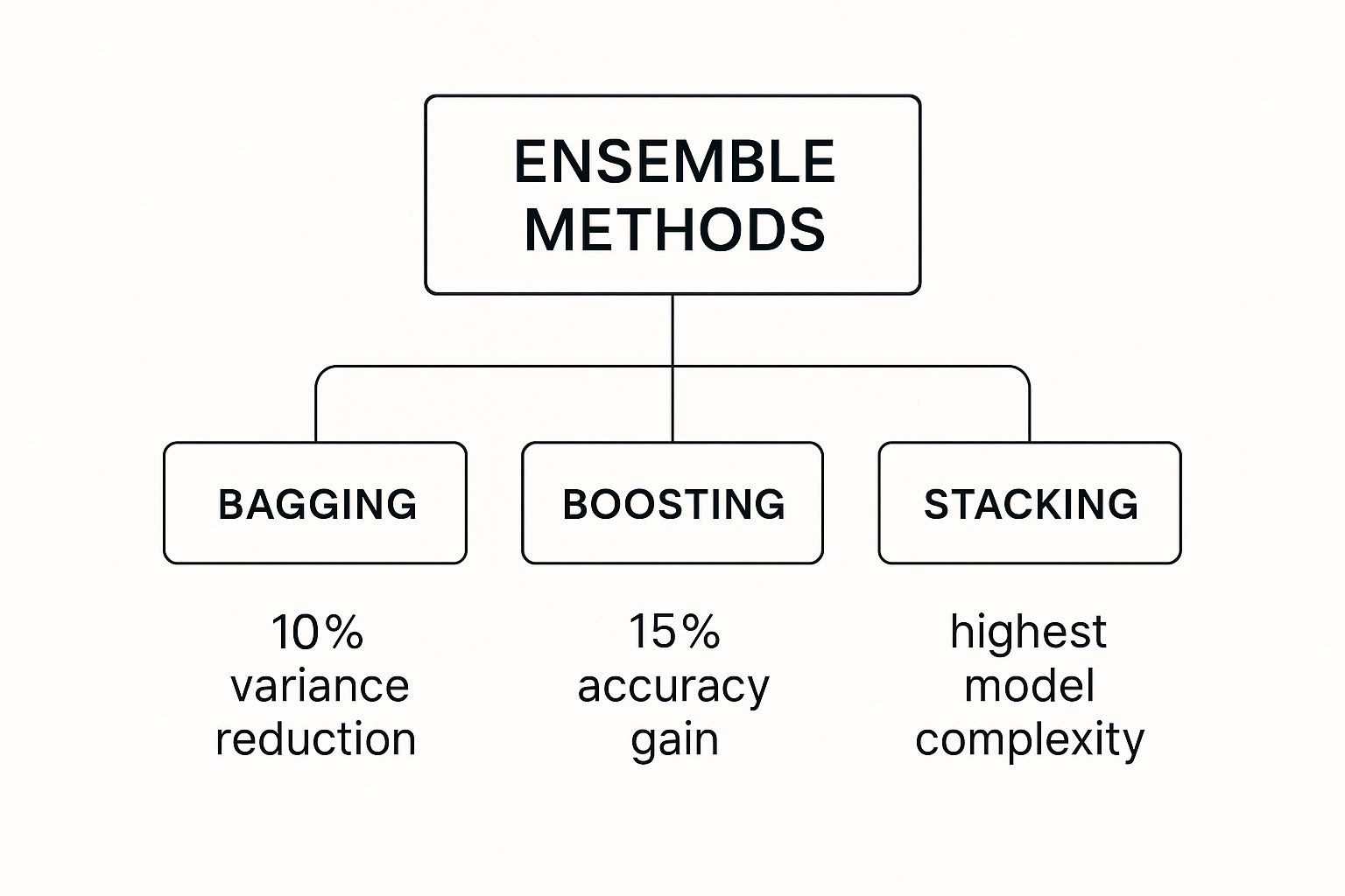
The infographic below shows where Stacking fits in the hierarchy of common ensemble methods machine learning, highlighting its power but also its added complexity.

As you can see, while Bagging and Boosting offer huge gains, Stacking represents the next level of model combination. It's often the go-to method when you need to squeeze out every last bit of performance, though it comes at the cost of being a bit more complex to set up.

How Stacking Works: The Two-Level Structure

Stacking, sometimes called stacked generalization, works in a two-level process. It’s a killer technique for boosting model accuracy, especially in competitive data science settings where even small performance gains can make a huge difference.

1. Level 0: Generate out-of-fold predictions for every training example by fitting each base estimator only on the other folds. These predictions form the meta-model’s training features. After meta-model training, refit the base estimators on the complete training set for inference.

   Level 1: Fit a regularized final estimator to the out-of-fold prediction matrix, optionally with selected original features. Evaluate the entire stack in an outer validation procedure when tuning choices were made from the same data.

2. Level 1 (Meta-Model): The predictions from these Level 0 models become the input features for a new, final model. We call this the meta-model or blender. Its entire job is to learn the optimal way to combine the predictions from the base learners.

The core idea behind Stacking isn't just to average predictions, but to learn the complex relationships between the outputs of strong, diverse models. The meta-model effectively figures out when to trust each base model and by how much.

A Practical Example: Predicting Real Estate Value

Let's make this real with a common problem: predicting a home's final sale price. A single model might struggle to capture all the different signals in the data, but with Stacking, we can build something far more robust.

The Actionable Insight: An investment firm wants to identify undervalued properties for its portfolio. They need the most accurate valuation model possible to maximize their return on investment.

• Level 0 Base Models:
  • Model A (XGBoost): Fantastic at capturing complex interactions between numerical features like square footage and lot size.
  • Model B (Ridge Regression): A simple linear model that provides a stable, regularized baseline prediction.
  • Model C (LightGBM): Another powerful gradient boosting model, but with a different tree-growth strategy that might spot patterns XGBoost missed.

We'd start by training each of these three models on our real estate data. The predictions they make for each house now become our new set of features.

• Level 1 Meta-Model:
  • Model D (Linear Regression): We then train a simple Linear Regression model. Its job isn't to predict house prices from the original data, but to learn the best coefficients (or weights) for combining the predictions from XGBoost, Ridge, and LightGBM.

A linear meta-model learns global coefficients for the base predictions; it does not learn property-specific switching unless the design supplies interactions or uses a nonlinear final estimator. Any added flexibility must be validated to avoid overfitting.

Avoiding the Pitfall of Data Leakage

One of the most critical parts of implementing Stacking correctly is avoiding data leakage. You absolutely cannot train the Level 0 models and the Level 1 meta-model on the exact same data. If you do, the meta-model will learn patterns that only exist in the training set and will fail miserably on new, unseen data.

The standard solution here is cross-validation. You split the training data into several folds (say, 5 folds). The Level 0 models are trained on four of the folds and then make predictions on the fifth "out-of-fold" part. You repeat this process for all folds until you have a clean set of predictions for the entire training set.

This ensures the meta-model learns from predictions made on data it has never seen during its training, making the final ensemble much more reliable. Yes, Stacking is computationally intensive, but for complex problems, it's an incredibly effective tool in the ensemble methods machine learning toolkit.

How to Choose the Right Ensemble Method

So, how do you pick the right tool for the job? Selecting the best ensemble method really comes down to what you're trying to achieve. You need to weigh the trade-offs between raw performance, how long you're willing to wait for training, and whether you need to explain why the model made its decision.

There’s no magic bullet, and the "best" technique depends entirely on the problem staring you in the face. It’s all about finding the right fit for your specific goals with ensemble methods machine learning.

Your Go-To Starting Point: Random Forest

For a lot of projects, your first stop should be Random Forest. Think of it as your reliable, all-purpose baseline.

It’s a bagging method that’s naturally robust, much less likely to overfit than a single decision tree, and it often gives you great results right out of the box with minimal tuning. It's the perfect benchmark to measure more complex models against.

When to Bring Out the Big Guns: Boosting and Stacking

If your main goal is squeezing every last drop of predictive accuracy out of your data—especially if it's structured or tabular—then it's time to look at boosting algorithms like XGBoost or LightGBM. These are the heavy hitters, designed to hunt down and correct errors by aggressively reducing bias. They can spot subtle patterns that bagging methods might just skim over.

But all that power comes with a catch. Boosted models are more sensitive to their settings and have a higher risk of overfitting if you aren't careful with tuning.

Stacking is the final boss. You save it for situations where you absolutely need to eke out that last fraction of a percent in performance, like in a modeling competition. It's a beast to set up and computationally expensive, but it can deliver state-of-the-art results by cleverly combining the unique strengths of completely different models.

Here are a few quick rules of thumb to guide you:

• Need speed and a solid baseline? Start with Random Forest.
• Chasing maximum accuracy on tabular data? Level up to XGBoost or LightGBM.
• Is interpretability a must-have? Random Forest is your friend. Its feature importance scores are far easier to unpack than a boosted model's inner workings.
• Fighting for the top of the leaderboard? Use Stacking to blend your best models into a powerhouse.

A Practical Comparison

To make the choice clearer, here’s a quick breakdown of how these methods stack up against each other based on common project needs.

Comparison of Major Ensemble Methods

Method	What it changes	Strength	Main risk
Bagging / Random Forest	Averages randomized fits	Often reduces variance and provides a strong nonlinear baseline	Compute cost; correlated trees; importance scores can mislead
Gradient-boosted trees	Adds learners stage by stage to optimize a loss	Strong performance on many tabular tasks	Sensitivity to validation, regularization, and leakage
Stacking	Learns a combination of out-of-fold base predictions	Can exploit complementary errors	Leakage, nested validation complexity, and operational cost

Choosing the right model is a fundamental skill, but it’s just one piece of the puzzle. For a bigger picture on building and validating high-quality models, our guide to mastering machine learning offers a deeper dive into the end-to-end workflow.

Frequently Asked Questions About Ensemble Methods

We’ve covered a lot of ground, but a few common questions always pop up when people start putting ensemble methods machine learning into practice. Let's tackle those head-on to clear up any lingering confusion.

Can I Combine Different Types of Models in an Ensemble?

Absolutely! In fact, that's the entire idea behind stacking.

This technique is designed to blend the strengths of completely different models—think a Random Forest, a Support Vector Machine, and a gradient boosting model all working together. A final "meta-model" then learns how to intelligently weigh the predictions from each one to produce a result that's often better than any single model could achieve on its own.

How Many Models Should I Use in an Ensemble?

There is no universal number. For averaging ensembles such as random forests, adding trees generally stabilizes the estimate rather than producing the same overfitting pattern as adding boosting rounds, although it increases compute and memory. For boosting, excessive rounds can overfit, so tune the learning-rate/rounds combination and use early stopping where appropriate. For voting and stacking, additional estimators help only when they add useful, sufficiently diverse signal. Plot validation performance and resource cost rather than relying on a fixed range.

Once your model is live, you can't just set it and forget it. Performance can drift. To learn how to keep your ensembles sharp in production, check out our guide on effective machine learning model monitoring.

Primary references

1. Scikit-learn: ensemble methods
2. Scikit-learn: stacking predictors
3. Scikit-learn: permutation importance
4. XGBoost parameter reference
5. Breiman: Random Forests
6. Friedman: Gradient Boosting Machine
7. Wolpert: Stacked Generalization

Fact-check record

Reviewed September 4, 2026. Removed universal accuracy claims; corrected weak-learner terminology, bias–variance framing, categorical support, feature-importance caveats, gradient mechanics, XGBoost parallelism, validation-based tuning, stacking leakage controls, and estimator-count guidance.

---