8 Time-Series Forecasting Techniques Compared

Unlocking the Power of Time: Exploring Time Series Analysis

Evaluate every method on future, unseen periods

Do not choose a forecasting model from in-sample fit or a generic ranking. Establish a seasonal-naive or otherwise appropriate baseline, preserve chronological order, and evaluate genuine forecasts on a holdout period or rolling-origin backtest. Match each test window to the operational forecast horizon, use metrics that fit the decision, and inspect calibration and failure modes.

ARIMA is useful when differencing and linear dependence adequately describe a univariate series. It is widely used as a baseline and for economic, demand, and operational forecasts, but historical price fit does not imply useful or profitable stock-price forecasting.

>Unlocking the Power of Time: Exploring Time Series Analysis

Evaluate every method on future, unseen periods

Do not choose a forecasting model from in-sample fit or a generic ranking. Establish a seasonal-naive or otherwise appropriate baseline, preserve chronological order, and evaluate genuine forecasts on a holdout period or rolling-origin backtest. Match each test window to the operational forecast horizon, use metrics that fit the decision, and inspect calibration and failure modes.

Inspect the series and residuals, consider structural breaks and seasonality, and use unit-root tests as evidence rather than a mechanical gate. ACF and PACF plots can suggest candidate orders, but compare candidates with information criteria and rolling out-of-sample forecasts. Use SARIMA/SARIMAX when seasonal structure or exogenous regressors belong in the specification.

>Unlocking the Power of Time: Exploring Time Series Analysis

Evaluate every method on future, unseen periods

Do not choose a forecasting model from in-sample fit or a generic ranking. Establish a seasonal-naive or otherwise appropriate baseline, preserve chronological order, and evaluate genuine forecasts on a holdout period or rolling-origin backtest. Match each test window to the operational forecast horizon, use metrics that fit the decision, and inspect calibration and failure modes.

ARIMA is useful when differencing and linear dependence adequately describe a univariate series. It is widely used as a baseline and for economic, demand, and operational forecasts, but historical price fit does not imply useful or profitable stock-price forecasting.

>Unlocking the Power of Time: Exploring Time Series Analysis

Evaluate every method on future, unseen periods

Do not choose a forecasting model from in-sample fit or a generic ranking. Establish a seasonal-naive or otherwise appropriate baseline, preserve chronological order, and evaluate genuine forecasts on a holdout period or rolling-origin backtest. Match each test window to the operational forecast horizon, use metrics that fit the decision, and inspect calibration and failure modes.

Prophet is an additive forecasting procedure with trend, seasonal, holiday, and optional regressor components. Its documentation says it works best when a series has strong seasonal effects and several seasons of history. Benchmark it against simpler baselines and alternatives on the actual forecast horizon.

>Unlocking the Power of Time: Exploring Time Series Analysis

Evaluate every method on future, unseen periods

Do not choose a forecasting model from in-sample fit or a generic ranking. Establish a seasonal-naive or otherwise appropriate baseline, preserve chronological order, and evaluate genuine forecasts on a holdout period or rolling-origin backtest. Match each test window to the operational forecast horizon, use metrics that fit the decision, and inspect calibration and failure modes.

ARIMA is useful when differencing and linear dependence adequately describe a univariate series. It is widely used as a baseline and for economic, demand, and operational forecasts, but historical price fit does not imply useful or profitable stock-price forecasting.

>Unlocking the Power of Time: Exploring Time Series Analysis

Evaluate every method on future, unseen periods

Do not choose a forecasting model from in-sample fit or a generic ranking. Establish a seasonal-naive or otherwise appropriate baseline, preserve chronological order, and evaluate genuine forecasts on a holdout period or rolling-origin backtest. Match each test window to the operational forecast horizon, use metrics that fit the decision, and inspect calibration and failure modes.

Inspect the series and residuals, consider structural breaks and seasonality, and use unit-root tests as evidence rather than a mechanical gate. ACF and PACF plots can suggest candidate orders, but compare candidates with information criteria and rolling out-of-sample forecasts. Use SARIMA/SARIMAX when seasonal structure or exogenous regressors belong in the specification.

>Unlocking the Power of Time: Exploring Time Series Analysis

Evaluate every method on future, unseen periods

Do not choose a forecasting model from in-sample fit or a generic ranking. Establish a seasonal-naive or otherwise appropriate baseline, preserve chronological order, and evaluate genuine forecasts on a holdout period or rolling-origin backtest. Match each test window to the operational forecast horizon, use metrics that fit the decision, and inspect calibration and failure modes.

ARIMA is useful when differencing and linear dependence adequately describe a univariate series. It is widely used as a baseline and for economic, demand, and operational forecasts, but historical price fit does not imply useful or profitable stock-price forecasting.

>Unlocking the Power of Time: Exploring Time Series Analysis

Evaluate every method on future, unseen periods

Do not choose a forecasting model from in-sample fit or a generic ranking. Establish a seasonal-naive or otherwise appropriate baseline, preserve chronological order, and evaluate genuine forecasts on a holdout period or rolling-origin backtest. Match each test window to the operational forecast horizon, use metrics that fit the decision, and inspect calibration and failure modes.

Fit all preprocessing, feature selection, and hyperparameter tuning inside each training window. Random cross-validation can leak future information; use expanding- or sliding-window evaluation for time-ordered data.

This listicle provides a concise overview of eight essential time series analysis techniques for data professionals, researchers, and strategists. Understanding these methods is crucial for extracting meaningful insights from temporal data, enabling more accurate predictions and better decision-making. Learn how techniques like ARIMA, Exponential Smoothing, Prophet, LSTM networks, Spectral Analysis, State Space Models, Vector Autoregression (VAR), and XGBoost can be applied to solve real-world problems. Each technique is presented with practical use cases to demonstrate its value in various domains.

1. ARIMA (AutoRegressive Integrated Moving Average)

ARIMA, short for AutoRegressive Integrated Moving Average, stands as a cornerstone in the realm of time series analysis techniques. It's a statistical model employed to understand and predict future points in a time series dataset. ARIMA leverages past values within the series itself to forecast future trends, making it particularly powerful for data exhibiting clear temporal dependencies. The model operates by combining three core components: autoregression (AR), integration (I), and moving average (MA). Autoregression captures the relationship between a data point and its own lagged values. Integration addresses the issue of non-stationarity in the data by differencing the series, essentially calculating the changes between consecutive observations. Finally, the moving average component accounts for the relationship between a data point and residual errors from a moving average model applied to lagged observations. An ARIMA model is typically denoted as ARIMA(p,d,q), where 'p' represents the autoregressive order, 'd' the degree of differencing, and 'q' the moving average order. These parameters are crucial for tailoring the model to the specific characteristics of the time series data. ARIMA models find wide applicability across various domains. For example, in economics, ARIMA is used for forecasting key indicators like GDP and unemployment rates. Financial analysts employ ARIMA for stock price prediction and market analysis. Retail businesses leverage it for sales forecasting, and utility companies utilize it for energy load prediction. The versatility of ARIMA stems from its ability to capture both seasonal and non-seasonal patterns, especially when extended to Seasonal ARIMA (SARIMA). This adaptability makes ARIMA a valuable tool for anyone working with time-dependent data. One of the key advantages of ARIMA is its well-established methodological foundation and strong theoretical backing. It provides a relatively interpretable framework compared to more complex, black-box methods, allowing users to gain insights into the underlying patterns driving the time series. Furthermore, ARIMA provides confidence intervals for forecasts, offering a measure of uncertainty associated with the predictions. However, ARIMA also has limitations. It assumes linear relationships within the data, and requires the time series to be stationary or transformed to achieve stationarity. Model selection, specifically determining the optimal p, d, and q parameters, can be challenging. Moreover, ARIMA struggles to capture complex non-linear patterns. For those working with time series analysis, several practical tips can aid in effective ARIMA implementation. Before applying ARIMA, it's crucial to test for stationarity using tests like the Augmented Dickey-Fuller test. Autocorrelation Function (ACF) and Partial Autocorrelation Function (PACF) plots provide valuable visual aids for identifying appropriate p and q values. Comparing multiple models using metrics such as AIC (Akaike Information Criterion) or BIC (Bayesian Information Criterion) helps in selecting the best-fitting model. Finally, when dealing with seasonal data, consider using the SARIMA extension. Learn more about ARIMA (AutoRegressive Integrated Moving Average) The work of George Box and Gwilym Jenkins in 1970 popularized ARIMA, and more recently, Rob Hyndman, author of "Forecasting: Principles and Practice," and the R package 'forecast' have contributed significantly to its widespread use. ARIMA’s robust theoretical foundation, coupled with its practical applicability, secures its position as a fundamental technique in the toolkit of any data scientist tackling time series analysis.

2. Exponential Smoothing Methods

Exponential smoothing methods represent a powerful family of time series analysis techniques specifically designed for forecasting. Their core principle lies in assigning exponentially decreasing weights to past observations, emphasizing the importance of recent data in predicting future values. This characteristic makes them particularly well-suited for capturing evolving trends and patterns in time series data. This approach earns its place on the list of essential time series analysis techniques due to its computational efficiency, ease of implementation, and ability to produce reliable short-term forecasts, even with limited historical data. How Exponential Smoothing Works: Unlike simple moving averages which give equal weight to all observations within a window, exponential smoothing assigns progressively smaller weights to older data points. The weight assigned to an observation is determined by a smoothing parameter, typically denoted by α (alpha), where 0 < α ≤ 1. A higher α value places more emphasis on recent observations, making the forecast more responsive to recent changes, while a lower α gives more weight to historical data, resulting in a smoother forecast. Variants of Exponential Smoothing: Several variants of exponential smoothing exist to address different characteristics of time series data:

• Simple Exponential Smoothing (SES): The most basic form, SES is suitable for time series data without clear trends or seasonality. It forecasts future values based on a weighted average of past observations, with weights decaying exponentially.
• Holt's Linear Method: This extension of SES incorporates a trend component, allowing it to model time series with a linear trend. It uses two smoothing parameters: one for the level and one for the trend.
• Holt-Winters Method: The most advanced variant, Holt-Winters accounts for both trend and seasonality. It employs three smoothing parameters: one for the level, one for the trend, and one for the seasonal component. This method offers two options for modeling seasonality: additive and multiplicative. Additive seasonality assumes that the seasonal fluctuations are constant over time, while multiplicative seasonality assumes that the fluctuations are proportional to the level of the time series.

Features and Benefits:

• Weighted Averaging: Exponentially decreasing weights allow the model to adapt to recent changes while still considering historical context.
• Handles Level, Trend, and Seasonality: Different variants cater to various time series characteristics, providing flexibility in modeling.
• State Space Formulation: Modern implementations often utilize a state space representation, which allows for calculating prediction intervals, quantifying the uncertainty associated with the forecasts.
• Adaptive Models: The smoothing parameters can be adjusted over time to emphasize more recent observations, making the model adaptive to changing patterns.

Pros:

• Computationally Efficient and Easy to Implement: Exponential smoothing methods are relatively simple to understand and implement, requiring minimal computational resources.
• Intuitive and Interpretable Parameters: The smoothing parameters have a clear interpretation, making it easier to understand how the model is behaving.
• Outliers and level shifts: Ordinary exponential-smoothing estimates can be distorted by unusual observations. Diagnose outliers and structural changes; use robust estimation or explicit intervention treatment when warranted.
• Data requirements: Simple variants are parsimonious, but seasonal models still need enough cycles to estimate and validate the seasonal pattern. Limited data does not guarantee reliable forecasts.

Cons:

• May Oversimplify Complex Temporal Dynamics: For highly complex time series with non-linear patterns, exponential smoothing might oversimplify the underlying dynamics.
• Less Effective for Long-Term Forecasting: Due to the emphasis on recent data, exponential smoothing is generally more suitable for short-term forecasting.
• Cannot Incorporate External Variables Easily: It's challenging to directly incorporate external factors (e.g., economic indicators) into the model.
• Struggle with Abrupt Pattern Changes: While adaptive methods can help, exponential smoothing can be slow to react to sudden and significant shifts in the time series pattern.

Examples of Successful Implementation:

• Inventory management and demand forecasting in supply chains: Predicting short-term demand to optimize inventory levels.
• Short-term sales predictions in retail: Forecasting sales for the upcoming week or month to inform staffing and promotional decisions.
• Tourism and hotel booking forecasts: Predicting occupancy rates to optimize pricing and resource allocation.
• Utility companies forecasting short-term consumption: Forecasting electricity or gas demand to manage production and distribution.

Tips for Effective Use:

• Choose the appropriate variant: Select the variant (SES, Holt's Linear, or Holt-Winters) based on the presence of trend and seasonality in the data.
• Optimize smoothing parameters: Use cross-validation or other optimization techniques to find the best values for the smoothing parameters.
• For Holt-Winters, consider both additive and multiplicative seasonality: Experiment with both types of seasonality to determine which one best fits the data.
• Regularly update models with new data: To maintain forecast accuracy, re-train or update the model periodically with new observations.

Popularized By: Charles C. Holt (1957), Peter Winters (1960), Rob Hyndman (ETS models implementation), and forecasting software like SAS and Oracle Demand Planning have all contributed to the widespread adoption of exponential smoothing methods.

3. Prophet

Prophet, a powerful time series analysis technique developed by Meta (formerly Facebook), stands out for its ability to generate high-quality forecasts, especially for data exhibiting complex seasonality and holiday effects. Its user-friendly nature and robust performance make it a valuable tool in the arsenal of any data scientist tackling time series forecasting challenges. This approach deserves its place on this list due to its unique combination of sophisticated modeling capabilities and ease of use, making accurate time series analysis accessible to a broader audience. Prophet implements an additive regression model, decomposing the time series into distinct components: trend, seasonality, and holidays. This decomposition allows for a more nuanced understanding of the underlying forces driving the data. The trend component captures the overall growth or decline over time, while the seasonality component models repeating patterns at different time scales (e.g., daily, weekly, yearly). Crucially, Prophet explicitly incorporates the impact of holidays and events, a feature often overlooked by other time series analysis techniques. How it works: Prophet utilizes a curve-fitting approach to model the trend component, automatically detecting changepoints where the rate of growth shifts. This automatic changepoint detection simplifies the modeling process and allows Prophet to adapt to evolving trends in the data. The seasonality component is modeled using Fourier series, allowing for flexible representation of complex seasonal patterns. Finally, the holiday component is incorporated by explicitly modeling the impact of known holidays and events, which are provided as input to the model. Features and Benefits:

• Decomposable Model: The separation of trend, seasonality, and holidays makes the model interpretable and allows for better understanding of the contributing factors.
• Automatic Changepoint Detection: Simplifies model building and adapts to changing trends.
• Multiple Seasonality: Handles various seasonal patterns simultaneously.
• Custom Holiday and Event Modeling: Incorporates the impact of specific events on the time series.
• Robust to Outliers and Missing Data: Provides reliable forecasts even with imperfect data.

Pros:

• User-Friendly: Requires minimal parameter tuning, making it accessible to users with varying levels of statistical expertise.
• Robust: Handles missing data and outliers effectively.
• Incorporates Domain Knowledge: Allows users to specify relevant holidays and events.
• Automatic Seasonality Handling: Detects and models seasonality at different time scales.

Cons:

• Overfitting Potential: Can sometimes overfit with too many changepoints, especially in datasets with high volatility.
• Sub-daily data: Prophet supports sub-daily series and daily seasonality. Regularly missing portions of each day need care because unconstrained seasonal components can behave poorly in unseen windows.
• External regressors: add_regressor supports additional predictors. Their values must be available for training and future dates, or forecast separately; uncertainty in a forecasted regressor propagates into the target forecast.
• Computational Intensity: Can be computationally expensive for very large datasets.

Examples of Successful Implementation:

• Forecasting user growth and engagement metrics at Meta: Prophet was originally developed to address Facebook's forecasting needs.
• Retail sales forecasting with holiday effects: Accurately predicting sales during peak seasons by accounting for holidays and promotional events.
• Website traffic prediction: Forecasting website traffic patterns based on historical data and seasonal trends.
• Capacity planning for cloud infrastructure services: Predicting resource demand and optimizing resource allocation.

Actionable Tips:

• Leverage Domain Expertise: Use your knowledge to specify relevant holidays and events.
• Control Changepoint Flexibility: Adjust the changepoint_prior_scale parameter to control the sensitivity to trend changes. Higher values allow for more flexibility, but increase the risk of overfitting.
• Transform for Multiplicative Patterns: Apply a logarithmic transformation to the data if you suspect multiplicative seasonality.
• Compare with Simpler Models: Benchmark against simpler time series models like ARIMA to avoid unnecessary complexity and potential overfitting.

Popularized By: Sean J. Taylor and Benjamin Letham (Facebook/Meta), Meta's Core Data Science team developed and popularized Prophet. Implementations are readily available in both R and Python. While a specific website link is not consistently advertised, searching for "Prophet Facebook" or "Prophet Time Series" will yield relevant resources, including documentation and tutorials. By leveraging Prophet's powerful features and adhering to these tips, data scientists, AI researchers, machine learning practitioners, IT leaders, and business executives can effectively tackle diverse time series analysis challenges and unlock valuable insights from their data. Its user-friendly design and robust performance empower even those without deep statistical expertise to generate high-quality forecasts, making it a valuable addition to any time series analysis toolkit.

4. Long Short-Term Memory Networks (LSTM)

State-space implementations can update the latent state using available observations and propagate it through missing periods when the software and specification support missing values. This is model-based treatment of missingness, not proof that the missing-data mechanism is ignorable.

>Unlocking the Power of Time: Exploring Time Series Analysis

Evaluate every method on future, unseen periods

Do not choose a forecasting model from in-sample fit or a generic ranking. Establish a seasonal-naive or otherwise appropriate baseline, preserve chronological order, and evaluate genuine forecasts on a holdout period or rolling-origin backtest. Match each test window to the operational forecast horizon, use metrics that fit the decision, and inspect calibration and failure modes.

ARIMA is useful when differencing and linear dependence adequately describe a univariate series. It is widely used as a baseline and for economic, demand, and operational forecasts, but historical price fit does not imply useful or profitable stock-price forecasting.

>Unlocking the Power of Time: Exploring Time Series Analysis

Evaluate every method on future, unseen periods

Do not choose a forecasting model from in-sample fit or a generic ranking. Establish a seasonal-naive or otherwise appropriate baseline, preserve chronological order, and evaluate genuine forecasts on a holdout period or rolling-origin backtest. Match each test window to the operational forecast horizon, use metrics that fit the decision, and inspect calibration and failure modes.

Inspect the series and residuals, consider structural breaks and seasonality, and use unit-root tests as evidence rather than a mechanical gate. ACF and PACF plots can suggest candidate orders, but compare candidates with information criteria and rolling out-of-sample forecasts. Use SARIMA/SARIMAX when seasonal structure or exogenous regressors belong in the specification.

>Unlocking the Power of Time: Exploring Time Series Analysis

Evaluate every method on future, unseen periods

Do not choose a forecasting model from in-sample fit or a generic ranking. Establish a seasonal-naive or otherwise appropriate baseline, preserve chronological order, and evaluate genuine forecasts on a holdout period or rolling-origin backtest. Match each test window to the operational forecast horizon, use metrics that fit the decision, and inspect calibration and failure modes.

ARIMA is useful when differencing and linear dependence adequately describe a univariate series. It is widely used as a baseline and for economic, demand, and operational forecasts, but historical price fit does not imply useful or profitable stock-price forecasting.

>Unlocking the Power of Time: Exploring Time Series Analysis

Evaluate every method on future, unseen periods

Do not choose a forecasting model from in-sample fit or a generic ranking. Establish a seasonal-naive or otherwise appropriate baseline, preserve chronological order, and evaluate genuine forecasts on a holdout period or rolling-origin backtest. Match each test window to the operational forecast horizon, use metrics that fit the decision, and inspect calibration and failure modes.

Prophet is an additive forecasting procedure with trend, seasonal, holiday, and optional regressor components. Its documentation says it works best when a series has strong seasonal effects and several seasons of history. Benchmark it against simpler baselines and alternatives on the actual forecast horizon.

>Unlocking the Power of Time: Exploring Time Series Analysis

Evaluate every method on future, unseen periods

Do not choose a forecasting model from in-sample fit or a generic ranking. Establish a seasonal-naive or otherwise appropriate baseline, preserve chronological order, and evaluate genuine forecasts on a holdout period or rolling-origin backtest. Match each test window to the operational forecast horizon, use metrics that fit the decision, and inspect calibration and failure modes.

ARIMA is useful when differencing and linear dependence adequately describe a univariate series. It is widely used as a baseline and for economic, demand, and operational forecasts, but historical price fit does not imply useful or profitable stock-price forecasting.

>Unlocking the Power of Time: Exploring Time Series Analysis

Evaluate every method on future, unseen periods

Do not choose a forecasting model from in-sample fit or a generic ranking. Establish a seasonal-naive or otherwise appropriate baseline, preserve chronological order, and evaluate genuine forecasts on a holdout period or rolling-origin backtest. Match each test window to the operational forecast horizon, use metrics that fit the decision, and inspect calibration and failure modes.

Inspect the series and residuals, consider structural breaks and seasonality, and use unit-root tests as evidence rather than a mechanical gate. ACF and PACF plots can suggest candidate orders, but compare candidates with information criteria and rolling out-of-sample forecasts. Use SARIMA/SARIMAX when seasonal structure or exogenous regressors belong in the specification.

>Unlocking the Power of Time: Exploring Time Series Analysis

Evaluate every method on future, unseen periods

Do not choose a forecasting model from in-sample fit or a generic ranking. Establish a seasonal-naive or otherwise appropriate baseline, preserve chronological order, and evaluate genuine forecasts on a holdout period or rolling-origin backtest. Match each test window to the operational forecast horizon, use metrics that fit the decision, and inspect calibration and failure modes.

ARIMA is useful when differencing and linear dependence adequately describe a univariate series. It is widely used as a baseline and for economic, demand, and operational forecasts, but historical price fit does not imply useful or profitable stock-price forecasting.

>Unlocking the Power of Time: Exploring Time Series Analysis

Evaluate every method on future, unseen periods

Do not choose a forecasting model from in-sample fit or a generic ranking. Establish a seasonal-naive or otherwise appropriate baseline, preserve chronological order, and evaluate genuine forecasts on a holdout period or rolling-origin backtest. Match each test window to the operational forecast horizon, use metrics that fit the decision, and inspect calibration and failure modes.

Fit all preprocessing, feature selection, and hyperparameter tuning inside each training window. Random cross-validation can leak future information; use expanding- or sliding-window evaluation for time-ordered data.

This listicle provides a concise overview of eight essential time series analysis techniques for data professionals, researchers, and strategists. Understanding these methods is crucial for extracting meaningful insights from temporal data, enabling more accurate predictions and better decision-making. Learn how techniques like ARIMA, Exponential Smoothing, Prophet, LSTM networks, Spectral Analysis, State Space Models, Vector Autoregression (VAR), and XGBoost can be applied to solve real-world problems. Each technique is presented with practical use cases to demonstrate its value in various domains.

1. ARIMA (AutoRegressive Integrated Moving Average)

ARIMA, short for AutoRegressive Integrated Moving Average, stands as a cornerstone in the realm of time series analysis techniques. It's a statistical model employed to understand and predict future points in a time series dataset. ARIMA leverages past values within the series itself to forecast future trends, making it particularly powerful for data exhibiting clear temporal dependencies. The model operates by combining three core components: autoregression (AR), integration (I), and moving average (MA). Autoregression captures the relationship between a data point and its own lagged values. Integration addresses the issue of non-stationarity in the data by differencing the series, essentially calculating the changes between consecutive observations. Finally, the moving average component accounts for the relationship between a data point and residual errors from a moving average model applied to lagged observations. An ARIMA model is typically denoted as ARIMA(p,d,q), where 'p' represents the autoregressive order, 'd' the degree of differencing, and 'q' the moving average order. These parameters are crucial for tailoring the model to the specific characteristics of the time series data. ARIMA models find wide applicability across various domains. For example, in economics, ARIMA is used for forecasting key indicators like GDP and unemployment rates. Financial analysts employ ARIMA for stock price prediction and market analysis. Retail businesses leverage it for sales forecasting, and utility companies utilize it for energy load prediction. The versatility of ARIMA stems from its ability to capture both seasonal and non-seasonal patterns, especially when extended to Seasonal ARIMA (SARIMA). This adaptability makes ARIMA a valuable tool for anyone working with time-dependent data. One of the key advantages of ARIMA is its well-established methodological foundation and strong theoretical backing. It provides a relatively interpretable framework compared to more complex, black-box methods, allowing users to gain insights into the underlying patterns driving the time series. Furthermore, ARIMA provides confidence intervals for forecasts, offering a measure of uncertainty associated with the predictions. However, ARIMA also has limitations. It assumes linear relationships within the data, and requires the time series to be stationary or transformed to achieve stationarity. Model selection, specifically determining the optimal p, d, and q parameters, can be challenging. Moreover, ARIMA struggles to capture complex non-linear patterns. For those working with time series analysis, several practical tips can aid in effective ARIMA implementation. Before applying ARIMA, it's crucial to test for stationarity using tests like the Augmented Dickey-Fuller test. Autocorrelation Function (ACF) and Partial Autocorrelation Function (PACF) plots provide valuable visual aids for identifying appropriate p and q values. Comparing multiple models using metrics such as AIC (Akaike Information Criterion) or BIC (Bayesian Information Criterion) helps in selecting the best-fitting model. Finally, when dealing with seasonal data, consider using the SARIMA extension. Learn more about ARIMA (AutoRegressive Integrated Moving Average) The work of George Box and Gwilym Jenkins in 1970 popularized ARIMA, and more recently, Rob Hyndman, author of "Forecasting: Principles and Practice," and the R package 'forecast' have contributed significantly to its widespread use. ARIMA’s robust theoretical foundation, coupled with its practical applicability, secures its position as a fundamental technique in the toolkit of any data scientist tackling time series analysis.

2. Exponential Smoothing Methods

Exponential smoothing methods represent a powerful family of time series analysis techniques specifically designed for forecasting. Their core principle lies in assigning exponentially decreasing weights to past observations, emphasizing the importance of recent data in predicting future values. This characteristic makes them particularly well-suited for capturing evolving trends and patterns in time series data. This approach earns its place on the list of essential time series analysis techniques due to its computational efficiency, ease of implementation, and ability to produce reliable short-term forecasts, even with limited historical data. How Exponential Smoothing Works: Unlike simple moving averages which give equal weight to all observations within a window, exponential smoothing assigns progressively smaller weights to older data points. The weight assigned to an observation is determined by a smoothing parameter, typically denoted by α (alpha), where 0 < α ≤ 1. A higher α value places more emphasis on recent observations, making the forecast more responsive to recent changes, while a lower α gives more weight to historical data, resulting in a smoother forecast. Variants of Exponential Smoothing: Several variants of exponential smoothing exist to address different characteristics of time series data:

• Simple Exponential Smoothing (SES): The most basic form, SES is suitable for time series data without clear trends or seasonality. It forecasts future values based on a weighted average of past observations, with weights decaying exponentially.
• Holt's Linear Method: This extension of SES incorporates a trend component, allowing it to model time series with a linear trend. It uses two smoothing parameters: one for the level and one for the trend.
• Holt-Winters Method: The most advanced variant, Holt-Winters accounts for both trend and seasonality. It employs three smoothing parameters: one for the level, one for the trend, and one for the seasonal component. This method offers two options for modeling seasonality: additive and multiplicative. Additive seasonality assumes that the seasonal fluctuations are constant over time, while multiplicative seasonality assumes that the fluctuations are proportional to the level of the time series.

Features and Benefits:

• Weighted Averaging: Exponentially decreasing weights allow the model to adapt to recent changes while still considering historical context.
• Handles Level, Trend, and Seasonality: Different variants cater to various time series characteristics, providing flexibility in modeling.
• State Space Formulation: Modern implementations often utilize a state space representation, which allows for calculating prediction intervals, quantifying the uncertainty associated with the forecasts.
• Adaptive Models: The smoothing parameters can be adjusted over time to emphasize more recent observations, making the model adaptive to changing patterns.

Pros:

• Computationally Efficient and Easy to Implement: Exponential smoothing methods are relatively simple to understand and implement, requiring minimal computational resources.
• Intuitive and Interpretable Parameters: The smoothing parameters have a clear interpretation, making it easier to understand how the model is behaving.
• Outliers and level shifts: Ordinary exponential-smoothing estimates can be distorted by unusual observations. Diagnose outliers and structural changes; use robust estimation or explicit intervention treatment when warranted.
• Data requirements: Simple variants are parsimonious, but seasonal models still need enough cycles to estimate and validate the seasonal pattern. Limited data does not guarantee reliable forecasts.

Cons:

• May Oversimplify Complex Temporal Dynamics: For highly complex time series with non-linear patterns, exponential smoothing might oversimplify the underlying dynamics.
• Less Effective for Long-Term Forecasting: Due to the emphasis on recent data, exponential smoothing is generally more suitable for short-term forecasting.
• Cannot Incorporate External Variables Easily: It's challenging to directly incorporate external factors (e.g., economic indicators) into the model.
• Struggle with Abrupt Pattern Changes: While adaptive methods can help, exponential smoothing can be slow to react to sudden and significant shifts in the time series pattern.

Examples of Successful Implementation:

• Inventory management and demand forecasting in supply chains: Predicting short-term demand to optimize inventory levels.
• Short-term sales predictions in retail: Forecasting sales for the upcoming week or month to inform staffing and promotional decisions.
• Tourism and hotel booking forecasts: Predicting occupancy rates to optimize pricing and resource allocation.
• Utility companies forecasting short-term consumption: Forecasting electricity or gas demand to manage production and distribution.

Tips for Effective Use:

• Choose the appropriate variant: Select the variant (SES, Holt's Linear, or Holt-Winters) based on the presence of trend and seasonality in the data.
• Optimize smoothing parameters: Use cross-validation or other optimization techniques to find the best values for the smoothing parameters.
• For Holt-Winters, consider both additive and multiplicative seasonality: Experiment with both types of seasonality to determine which one best fits the data.
• Regularly update models with new data: To maintain forecast accuracy, re-train or update the model periodically with new observations.

Popularized By: Charles C. Holt (1957), Peter Winters (1960), Rob Hyndman (ETS models implementation), and forecasting software like SAS and Oracle Demand Planning have all contributed to the widespread adoption of exponential smoothing methods.

3. Prophet

Prophet, a powerful time series analysis technique developed by Meta (formerly Facebook), stands out for its ability to generate high-quality forecasts, especially for data exhibiting complex seasonality and holiday effects. Its user-friendly nature and robust performance make it a valuable tool in the arsenal of any data scientist tackling time series forecasting challenges. This approach deserves its place on this list due to its unique combination of sophisticated modeling capabilities and ease of use, making accurate time series analysis accessible to a broader audience. Prophet implements an additive regression model, decomposing the time series into distinct components: trend, seasonality, and holidays. This decomposition allows for a more nuanced understanding of the underlying forces driving the data. The trend component captures the overall growth or decline over time, while the seasonality component models repeating patterns at different time scales (e.g., daily, weekly, yearly). Crucially, Prophet explicitly incorporates the impact of holidays and events, a feature often overlooked by other time series analysis techniques. How it works: Prophet utilizes a curve-fitting approach to model the trend component, automatically detecting changepoints where the rate of growth shifts. This automatic changepoint detection simplifies the modeling process and allows Prophet to adapt to evolving trends in the data. The seasonality component is modeled using Fourier series, allowing for flexible representation of complex seasonal patterns. Finally, the holiday component is incorporated by explicitly modeling the impact of known holidays and events, which are provided as input to the model. Features and Benefits:

• Decomposable Model: The separation of trend, seasonality, and holidays makes the model interpretable and allows for better understanding of the contributing factors.
• Automatic Changepoint Detection: Simplifies model building and adapts to changing trends.
• Multiple Seasonality: Handles various seasonal patterns simultaneously.
• Custom Holiday and Event Modeling: Incorporates the impact of specific events on the time series.
• Robust to Outliers and Missing Data: Provides reliable forecasts even with imperfect data.

Pros:

• User-Friendly: Requires minimal parameter tuning, making it accessible to users with varying levels of statistical expertise.
• Robust: Handles missing data and outliers effectively.
• Incorporates Domain Knowledge: Allows users to specify relevant holidays and events.
• Automatic Seasonality Handling: Detects and models seasonality at different time scales.

Cons:

• Overfitting Potential: Can sometimes overfit with too many changepoints, especially in datasets with high volatility.
• Sub-daily data: Prophet supports sub-daily series and daily seasonality. Regularly missing portions of each day need care because unconstrained seasonal components can behave poorly in unseen windows.
• External regressors: add_regressor supports additional predictors. Their values must be available for training and future dates, or forecast separately; uncertainty in a forecasted regressor propagates into the target forecast.
• Computational Intensity: Can be computationally expensive for very large datasets.

Examples of Successful Implementation:

• Forecasting user growth and engagement metrics at Meta: Prophet was originally developed to address Facebook's forecasting needs.
• Retail sales forecasting with holiday effects: Accurately predicting sales during peak seasons by accounting for holidays and promotional events.
• Website traffic prediction: Forecasting website traffic patterns based on historical data and seasonal trends.
• Capacity planning for cloud infrastructure services: Predicting resource demand and optimizing resource allocation.

Actionable Tips:

• Leverage Domain Expertise: Use your knowledge to specify relevant holidays and events.
• Control Changepoint Flexibility: Adjust the changepoint_prior_scale parameter to control the sensitivity to trend changes. Higher values allow for more flexibility, but increase the risk of overfitting.
• Transform for Multiplicative Patterns: Apply a logarithmic transformation to the data if you suspect multiplicative seasonality.
• Compare with Simpler Models: Benchmark against simpler time series models like ARIMA to avoid unnecessary complexity and potential overfitting.

Popularized By: Sean J. Taylor and Benjamin Letham (Facebook/Meta), Meta's Core Data Science team developed and popularized Prophet. Implementations are readily available in both R and Python. While a specific website link is not consistently advertised, searching for "Prophet Facebook" or "Prophet Time Series" will yield relevant resources, including documentation and tutorials. By leveraging Prophet's powerful features and adhering to these tips, data scientists, AI researchers, machine learning practitioners, IT leaders, and business executives can effectively tackle diverse time series analysis challenges and unlock valuable insights from their data. Its user-friendly design and robust performance empower even those without deep statistical expertise to generate high-quality forecasts, making it a valuable addition to any time series analysis toolkit.

4. Long Short-Term Memory Networks (LSTM)

Explore the Data4AI archive for related explanations of feature engineering, validation, anomaly detection, and machine-learning operations.

>Unlocking the Power of Time: Exploring Time Series Analysis

Evaluate every method on future, unseen periods

Do not choose a forecasting model from in-sample fit or a generic ranking. Establish a seasonal-naive or otherwise appropriate baseline, preserve chronological order, and evaluate genuine forecasts on a holdout period or rolling-origin backtest. Match each test window to the operational forecast horizon, use metrics that fit the decision, and inspect calibration and failure modes.

ARIMA is useful when differencing and linear dependence adequately describe a univariate series. It is widely used as a baseline and for economic, demand, and operational forecasts, but historical price fit does not imply useful or profitable stock-price forecasting.

>Unlocking the Power of Time: Exploring Time Series Analysis

Evaluate every method on future, unseen periods

Do not choose a forecasting model from in-sample fit or a generic ranking. Establish a seasonal-naive or otherwise appropriate baseline, preserve chronological order, and evaluate genuine forecasts on a holdout period or rolling-origin backtest. Match each test window to the operational forecast horizon, use metrics that fit the decision, and inspect calibration and failure modes.

Inspect the series and residuals, consider structural breaks and seasonality, and use unit-root tests as evidence rather than a mechanical gate. ACF and PACF plots can suggest candidate orders, but compare candidates with information criteria and rolling out-of-sample forecasts. Use SARIMA/SARIMAX when seasonal structure or exogenous regressors belong in the specification.

>Unlocking the Power of Time: Exploring Time Series Analysis

Evaluate every method on future, unseen periods

Do not choose a forecasting model from in-sample fit or a generic ranking. Establish a seasonal-naive or otherwise appropriate baseline, preserve chronological order, and evaluate genuine forecasts on a holdout period or rolling-origin backtest. Match each test window to the operational forecast horizon, use metrics that fit the decision, and inspect calibration and failure modes.

ARIMA is useful when differencing and linear dependence adequately describe a univariate series. It is widely used as a baseline and for economic, demand, and operational forecasts, but historical price fit does not imply useful or profitable stock-price forecasting.

>Unlocking the Power of Time: Exploring Time Series Analysis

Evaluate every method on future, unseen periods

Do not choose a forecasting model from in-sample fit or a generic ranking. Establish a seasonal-naive or otherwise appropriate baseline, preserve chronological order, and evaluate genuine forecasts on a holdout period or rolling-origin backtest. Match each test window to the operational forecast horizon, use metrics that fit the decision, and inspect calibration and failure modes.

Prophet is an additive forecasting procedure with trend, seasonal, holiday, and optional regressor components. Its documentation says it works best when a series has strong seasonal effects and several seasons of history. Benchmark it against simpler baselines and alternatives on the actual forecast horizon.

>Unlocking the Power of Time: Exploring Time Series Analysis

Evaluate every method on future, unseen periods

Do not choose a forecasting model from in-sample fit or a generic ranking. Establish a seasonal-naive or otherwise appropriate baseline, preserve chronological order, and evaluate genuine forecasts on a holdout period or rolling-origin backtest. Match each test window to the operational forecast horizon, use metrics that fit the decision, and inspect calibration and failure modes.

ARIMA is useful when differencing and linear dependence adequately describe a univariate series. It is widely used as a baseline and for economic, demand, and operational forecasts, but historical price fit does not imply useful or profitable stock-price forecasting.

>Unlocking the Power of Time: Exploring Time Series Analysis

Evaluate every method on future, unseen periods

Do not choose a forecasting model from in-sample fit or a generic ranking. Establish a seasonal-naive or otherwise appropriate baseline, preserve chronological order, and evaluate genuine forecasts on a holdout period or rolling-origin backtest. Match each test window to the operational forecast horizon, use metrics that fit the decision, and inspect calibration and failure modes.

Inspect the series and residuals, consider structural breaks and seasonality, and use unit-root tests as evidence rather than a mechanical gate. ACF and PACF plots can suggest candidate orders, but compare candidates with information criteria and rolling out-of-sample forecasts. Use SARIMA/SARIMAX when seasonal structure or exogenous regressors belong in the specification.

>Unlocking the Power of Time: Exploring Time Series Analysis

Evaluate every method on future, unseen periods

Do not choose a forecasting model from in-sample fit or a generic ranking. Establish a seasonal-naive or otherwise appropriate baseline, preserve chronological order, and evaluate genuine forecasts on a holdout period or rolling-origin backtest. Match each test window to the operational forecast horizon, use metrics that fit the decision, and inspect calibration and failure modes.

ARIMA is useful when differencing and linear dependence adequately describe a univariate series. It is widely used as a baseline and for economic, demand, and operational forecasts, but historical price fit does not imply useful or profitable stock-price forecasting.

>Unlocking the Power of Time: Exploring Time Series Analysis

Evaluate every method on future, unseen periods

Do not choose a forecasting model from in-sample fit or a generic ranking. Establish a seasonal-naive or otherwise appropriate baseline, preserve chronological order, and evaluate genuine forecasts on a holdout period or rolling-origin backtest. Match each test window to the operational forecast horizon, use metrics that fit the decision, and inspect calibration and failure modes.

Fit all preprocessing, feature selection, and hyperparameter tuning inside each training window. Random cross-validation can leak future information; use expanding- or sliding-window evaluation for time-ordered data.

This listicle provides a concise overview of eight essential time series analysis techniques for data professionals, researchers, and strategists. Understanding these methods is crucial for extracting meaningful insights from temporal data, enabling more accurate predictions and better decision-making. Learn how techniques like ARIMA, Exponential Smoothing, Prophet, LSTM networks, Spectral Analysis, State Space Models, Vector Autoregression (VAR), and XGBoost can be applied to solve real-world problems. Each technique is presented with practical use cases to demonstrate its value in various domains.

1. ARIMA (AutoRegressive Integrated Moving Average)

ARIMA, short for AutoRegressive Integrated Moving Average, stands as a cornerstone in the realm of time series analysis techniques. It's a statistical model employed to understand and predict future points in a time series dataset. ARIMA leverages past values within the series itself to forecast future trends, making it particularly powerful for data exhibiting clear temporal dependencies. The model operates by combining three core components: autoregression (AR), integration (I), and moving average (MA). Autoregression captures the relationship between a data point and its own lagged values. Integration addresses the issue of non-stationarity in the data by differencing the series, essentially calculating the changes between consecutive observations. Finally, the moving average component accounts for the relationship between a data point and residual errors from a moving average model applied to lagged observations. An ARIMA model is typically denoted as ARIMA(p,d,q), where 'p' represents the autoregressive order, 'd' the degree of differencing, and 'q' the moving average order. These parameters are crucial for tailoring the model to the specific characteristics of the time series data. ARIMA models find wide applicability across various domains. For example, in economics, ARIMA is used for forecasting key indicators like GDP and unemployment rates. Financial analysts employ ARIMA for stock price prediction and market analysis. Retail businesses leverage it for sales forecasting, and utility companies utilize it for energy load prediction. The versatility of ARIMA stems from its ability to capture both seasonal and non-seasonal patterns, especially when extended to Seasonal ARIMA (SARIMA). This adaptability makes ARIMA a valuable tool for anyone working with time-dependent data. One of the key advantages of ARIMA is its well-established methodological foundation and strong theoretical backing. It provides a relatively interpretable framework compared to more complex, black-box methods, allowing users to gain insights into the underlying patterns driving the time series. Furthermore, ARIMA provides confidence intervals for forecasts, offering a measure of uncertainty associated with the predictions. However, ARIMA also has limitations. It assumes linear relationships within the data, and requires the time series to be stationary or transformed to achieve stationarity. Model selection, specifically determining the optimal p, d, and q parameters, can be challenging. Moreover, ARIMA struggles to capture complex non-linear patterns. For those working with time series analysis, several practical tips can aid in effective ARIMA implementation. Before applying ARIMA, it's crucial to test for stationarity using tests like the Augmented Dickey-Fuller test. Autocorrelation Function (ACF) and Partial Autocorrelation Function (PACF) plots provide valuable visual aids for identifying appropriate p and q values. Comparing multiple models using metrics such as AIC (Akaike Information Criterion) or BIC (Bayesian Information Criterion) helps in selecting the best-fitting model. Finally, when dealing with seasonal data, consider using the SARIMA extension. Learn more about ARIMA (AutoRegressive Integrated Moving Average) The work of George Box and Gwilym Jenkins in 1970 popularized ARIMA, and more recently, Rob Hyndman, author of "Forecasting: Principles and Practice," and the R package 'forecast' have contributed significantly to its widespread use. ARIMA’s robust theoretical foundation, coupled with its practical applicability, secures its position as a fundamental technique in the toolkit of any data scientist tackling time series analysis.

2. Exponential Smoothing Methods

Exponential smoothing methods represent a powerful family of time series analysis techniques specifically designed for forecasting. Their core principle lies in assigning exponentially decreasing weights to past observations, emphasizing the importance of recent data in predicting future values. This characteristic makes them particularly well-suited for capturing evolving trends and patterns in time series data. This approach earns its place on the list of essential time series analysis techniques due to its computational efficiency, ease of implementation, and ability to produce reliable short-term forecasts, even with limited historical data. How Exponential Smoothing Works: Unlike simple moving averages which give equal weight to all observations within a window, exponential smoothing assigns progressively smaller weights to older data points. The weight assigned to an observation is determined by a smoothing parameter, typically denoted by α (alpha), where 0 < α ≤ 1. A higher α value places more emphasis on recent observations, making the forecast more responsive to recent changes, while a lower α gives more weight to historical data, resulting in a smoother forecast. Variants of Exponential Smoothing: Several variants of exponential smoothing exist to address different characteristics of time series data:

• Simple Exponential Smoothing (SES): The most basic form, SES is suitable for time series data without clear trends or seasonality. It forecasts future values based on a weighted average of past observations, with weights decaying exponentially.
• Holt's Linear Method: This extension of SES incorporates a trend component, allowing it to model time series with a linear trend. It uses two smoothing parameters: one for the level and one for the trend.
• Holt-Winters Method: The most advanced variant, Holt-Winters accounts for both trend and seasonality. It employs three smoothing parameters: one for the level, one for the trend, and one for the seasonal component. This method offers two options for modeling seasonality: additive and multiplicative. Additive seasonality assumes that the seasonal fluctuations are constant over time, while multiplicative seasonality assumes that the fluctuations are proportional to the level of the time series.

Features and Benefits:

• Weighted Averaging: Exponentially decreasing weights allow the model to adapt to recent changes while still considering historical context.
• Handles Level, Trend, and Seasonality: Different variants cater to various time series characteristics, providing flexibility in modeling.
• State Space Formulation: Modern implementations often utilize a state space representation, which allows for calculating prediction intervals, quantifying the uncertainty associated with the forecasts.
• Adaptive Models: The smoothing parameters can be adjusted over time to emphasize more recent observations, making the model adaptive to changing patterns.

Pros:

• Computationally Efficient and Easy to Implement: Exponential smoothing methods are relatively simple to understand and implement, requiring minimal computational resources.
• Intuitive and Interpretable Parameters: The smoothing parameters have a clear interpretation, making it easier to understand how the model is behaving.
• Outliers and level shifts: Ordinary exponential-smoothing estimates can be distorted by unusual observations. Diagnose outliers and structural changes; use robust estimation or explicit intervention treatment when warranted.
• Data requirements: Simple variants are parsimonious, but seasonal models still need enough cycles to estimate and validate the seasonal pattern. Limited data does not guarantee reliable forecasts.

Cons:

• May Oversimplify Complex Temporal Dynamics: For highly complex time series with non-linear patterns, exponential smoothing might oversimplify the underlying dynamics.
• Less Effective for Long-Term Forecasting: Due to the emphasis on recent data, exponential smoothing is generally more suitable for short-term forecasting.
• Cannot Incorporate External Variables Easily: It's challenging to directly incorporate external factors (e.g., economic indicators) into the model.
• Struggle with Abrupt Pattern Changes: While adaptive methods can help, exponential smoothing can be slow to react to sudden and significant shifts in the time series pattern.

Examples of Successful Implementation:

• Inventory management and demand forecasting in supply chains: Predicting short-term demand to optimize inventory levels.
• Short-term sales predictions in retail: Forecasting sales for the upcoming week or month to inform staffing and promotional decisions.
• Tourism and hotel booking forecasts: Predicting occupancy rates to optimize pricing and resource allocation.
• Utility companies forecasting short-term consumption: Forecasting electricity or gas demand to manage production and distribution.

Tips for Effective Use:

• Choose the appropriate variant: Select the variant (SES, Holt's Linear, or Holt-Winters) based on the presence of trend and seasonality in the data.
• Optimize smoothing parameters: Use cross-validation or other optimization techniques to find the best values for the smoothing parameters.
• For Holt-Winters, consider both additive and multiplicative seasonality: Experiment with both types of seasonality to determine which one best fits the data.
• Regularly update models with new data: To maintain forecast accuracy, re-train or update the model periodically with new observations.

Popularized By: Charles C. Holt (1957), Peter Winters (1960), Rob Hyndman (ETS models implementation), and forecasting software like SAS and Oracle Demand Planning have all contributed to the widespread adoption of exponential smoothing methods.

3. Prophet

Prophet, a powerful time series analysis technique developed by Meta (formerly Facebook), stands out for its ability to generate high-quality forecasts, especially for data exhibiting complex seasonality and holiday effects. Its user-friendly nature and robust performance make it a valuable tool in the arsenal of any data scientist tackling time series forecasting challenges. This approach deserves its place on this list due to its unique combination of sophisticated modeling capabilities and ease of use, making accurate time series analysis accessible to a broader audience. Prophet implements an additive regression model, decomposing the time series into distinct components: trend, seasonality, and holidays. This decomposition allows for a more nuanced understanding of the underlying forces driving the data. The trend component captures the overall growth or decline over time, while the seasonality component models repeating patterns at different time scales (e.g., daily, weekly, yearly). Crucially, Prophet explicitly incorporates the impact of holidays and events, a feature often overlooked by other time series analysis techniques. How it works: Prophet utilizes a curve-fitting approach to model the trend component, automatically detecting changepoints where the rate of growth shifts. This automatic changepoint detection simplifies the modeling process and allows Prophet to adapt to evolving trends in the data. The seasonality component is modeled using Fourier series, allowing for flexible representation of complex seasonal patterns. Finally, the holiday component is incorporated by explicitly modeling the impact of known holidays and events, which are provided as input to the model. Features and Benefits:

• Decomposable Model: The separation of trend, seasonality, and holidays makes the model interpretable and allows for better understanding of the contributing factors.
• Automatic Changepoint Detection: Simplifies model building and adapts to changing trends.
• Multiple Seasonality: Handles various seasonal patterns simultaneously.
• Custom Holiday and Event Modeling: Incorporates the impact of specific events on the time series.
• Robust to Outliers and Missing Data: Provides reliable forecasts even with imperfect data.

Pros:

• User-Friendly: Requires minimal parameter tuning, making it accessible to users with varying levels of statistical expertise.
• Robust: Handles missing data and outliers effectively.
• Incorporates Domain Knowledge: Allows users to specify relevant holidays and events.
• Automatic Seasonality Handling: Detects and models seasonality at different time scales.

Cons:

• Overfitting Potential: Can sometimes overfit with too many changepoints, especially in datasets with high volatility.
• Sub-daily data: Prophet supports sub-daily series and daily seasonality. Regularly missing portions of each day need care because unconstrained seasonal components can behave poorly in unseen windows.
• External regressors: add_regressor supports additional predictors. Their values must be available for training and future dates, or forecast separately; uncertainty in a forecasted regressor propagates into the target forecast.
• Computational Intensity: Can be computationally expensive for very large datasets.

Examples of Successful Implementation:

• Forecasting user growth and engagement metrics at Meta: Prophet was originally developed to address Facebook's forecasting needs.
• Retail sales forecasting with holiday effects: Accurately predicting sales during peak seasons by accounting for holidays and promotional events.
• Website traffic prediction: Forecasting website traffic patterns based on historical data and seasonal trends.
• Capacity planning for cloud infrastructure services: Predicting resource demand and optimizing resource allocation.

Actionable Tips:

• Leverage Domain Expertise: Use your knowledge to specify relevant holidays and events.
• Control Changepoint Flexibility: Adjust the changepoint_prior_scale parameter to control the sensitivity to trend changes. Higher values allow for more flexibility, but increase the risk of overfitting.
• Transform for Multiplicative Patterns: Apply a logarithmic transformation to the data if you suspect multiplicative seasonality.
• Compare with Simpler Models: Benchmark against simpler time series models like ARIMA to avoid unnecessary complexity and potential overfitting.

Popularized By: Sean J. Taylor and Benjamin Letham (Facebook/Meta), Meta's Core Data Science team developed and popularized Prophet. Implementations are readily available in both R and Python. While a specific website link is not consistently advertised, searching for "Prophet Facebook" or "Prophet Time Series" will yield relevant resources, including documentation and tutorials. By leveraging Prophet's powerful features and adhering to these tips, data scientists, AI researchers, machine learning practitioners, IT leaders, and business executives can effectively tackle diverse time series analysis challenges and unlock valuable insights from their data. Its user-friendly design and robust performance empower even those without deep statistical expertise to generate high-quality forecasts, making it a valuable addition to any time series analysis toolkit.

4. Long Short-Term Memory Networks (LSTM)

State-space implementations can update the latent state using available observations and propagate it through missing periods when the software and specification support missing values. This is model-based treatment of missingness, not proof that the missing-data mechanism is ignorable.

>Unlocking the Power of Time: Exploring Time Series Analysis

Evaluate every method on future, unseen periods

Do not choose a forecasting model from in-sample fit or a generic ranking. Establish a seasonal-naive or otherwise appropriate baseline, preserve chronological order, and evaluate genuine forecasts on a holdout period or rolling-origin backtest. Match each test window to the operational forecast horizon, use metrics that fit the decision, and inspect calibration and failure modes.

ARIMA is useful when differencing and linear dependence adequately describe a univariate series. It is widely used as a baseline and for economic, demand, and operational forecasts, but historical price fit does not imply useful or profitable stock-price forecasting.

>Unlocking the Power of Time: Exploring Time Series Analysis

Evaluate every method on future, unseen periods

Do not choose a forecasting model from in-sample fit or a generic ranking. Establish a seasonal-naive or otherwise appropriate baseline, preserve chronological order, and evaluate genuine forecasts on a holdout period or rolling-origin backtest. Match each test window to the operational forecast horizon, use metrics that fit the decision, and inspect calibration and failure modes.

Inspect the series and residuals, consider structural breaks and seasonality, and use unit-root tests as evidence rather than a mechanical gate. ACF and PACF plots can suggest candidate orders, but compare candidates with information criteria and rolling out-of-sample forecasts. Use SARIMA/SARIMAX when seasonal structure or exogenous regressors belong in the specification.

>Unlocking the Power of Time: Exploring Time Series Analysis

Evaluate every method on future, unseen periods

Do not choose a forecasting model from in-sample fit or a generic ranking. Establish a seasonal-naive or otherwise appropriate baseline, preserve chronological order, and evaluate genuine forecasts on a holdout period or rolling-origin backtest. Match each test window to the operational forecast horizon, use metrics that fit the decision, and inspect calibration and failure modes.

ARIMA is useful when differencing and linear dependence adequately describe a univariate series. It is widely used as a baseline and for economic, demand, and operational forecasts, but historical price fit does not imply useful or profitable stock-price forecasting.

>Unlocking the Power of Time: Exploring Time Series Analysis

Evaluate every method on future, unseen periods

Do not choose a forecasting model from in-sample fit or a generic ranking. Establish a seasonal-naive or otherwise appropriate baseline, preserve chronological order, and evaluate genuine forecasts on a holdout period or rolling-origin backtest. Match each test window to the operational forecast horizon, use metrics that fit the decision, and inspect calibration and failure modes.

Prophet is an additive forecasting procedure with trend, seasonal, holiday, and optional regressor components. Its documentation says it works best when a series has strong seasonal effects and several seasons of history. Benchmark it against simpler baselines and alternatives on the actual forecast horizon.

>Unlocking the Power of Time: Exploring Time Series Analysis

Evaluate every method on future, unseen periods

Do not choose a forecasting model from in-sample fit or a generic ranking. Establish a seasonal-naive or otherwise appropriate baseline, preserve chronological order, and evaluate genuine forecasts on a holdout period or rolling-origin backtest. Match each test window to the operational forecast horizon, use metrics that fit the decision, and inspect calibration and failure modes.

ARIMA is useful when differencing and linear dependence adequately describe a univariate series. It is widely used as a baseline and for economic, demand, and operational forecasts, but historical price fit does not imply useful or profitable stock-price forecasting.

>Unlocking the Power of Time: Exploring Time Series Analysis

Evaluate every method on future, unseen periods

Do not choose a forecasting model from in-sample fit or a generic ranking. Establish a seasonal-naive or otherwise appropriate baseline, preserve chronological order, and evaluate genuine forecasts on a holdout period or rolling-origin backtest. Match each test window to the operational forecast horizon, use metrics that fit the decision, and inspect calibration and failure modes.

Inspect the series and residuals, consider structural breaks and seasonality, and use unit-root tests as evidence rather than a mechanical gate. ACF and PACF plots can suggest candidate orders, but compare candidates with information criteria and rolling out-of-sample forecasts. Use SARIMA/SARIMAX when seasonal structure or exogenous regressors belong in the specification.

>Unlocking the Power of Time: Exploring Time Series Analysis

Evaluate every method on future, unseen periods

Do not choose a forecasting model from in-sample fit or a generic ranking. Establish a seasonal-naive or otherwise appropriate baseline, preserve chronological order, and evaluate genuine forecasts on a holdout period or rolling-origin backtest. Match each test window to the operational forecast horizon, use metrics that fit the decision, and inspect calibration and failure modes.

ARIMA is useful when differencing and linear dependence adequately describe a univariate series. It is widely used as a baseline and for economic, demand, and operational forecasts, but historical price fit does not imply useful or profitable stock-price forecasting.

>Unlocking the Power of Time: Exploring Time Series Analysis

Evaluate every method on future, unseen periods

Do not choose a forecasting model from in-sample fit or a generic ranking. Establish a seasonal-naive or otherwise appropriate baseline, preserve chronological order, and evaluate genuine forecasts on a holdout period or rolling-origin backtest. Match each test window to the operational forecast horizon, use metrics that fit the decision, and inspect calibration and failure modes.

Fit all preprocessing, feature selection, and hyperparameter tuning inside each training window. Random cross-validation can leak future information; use expanding- or sliding-window evaluation for time-ordered data.

This listicle provides a concise overview of eight essential time series analysis techniques for data professionals, researchers, and strategists. Understanding these methods is crucial for extracting meaningful insights from temporal data, enabling more accurate predictions and better decision-making. Learn how techniques like ARIMA, Exponential Smoothing, Prophet, LSTM networks, Spectral Analysis, State Space Models, Vector Autoregression (VAR), and XGBoost can be applied to solve real-world problems. Each technique is presented with practical use cases to demonstrate its value in various domains.

1. ARIMA (AutoRegressive Integrated Moving Average)

ARIMA, short for AutoRegressive Integrated Moving Average, stands as a cornerstone in the realm of time series analysis techniques. It's a statistical model employed to understand and predict future points in a time series dataset. ARIMA leverages past values within the series itself to forecast future trends, making it particularly powerful for data exhibiting clear temporal dependencies. The model operates by combining three core components: autoregression (AR), integration (I), and moving average (MA). Autoregression captures the relationship between a data point and its own lagged values. Integration addresses the issue of non-stationarity in the data by differencing the series, essentially calculating the changes between consecutive observations. Finally, the moving average component accounts for the relationship between a data point and residual errors from a moving average model applied to lagged observations. An ARIMA model is typically denoted as ARIMA(p,d,q), where 'p' represents the autoregressive order, 'd' the degree of differencing, and 'q' the moving average order. These parameters are crucial for tailoring the model to the specific characteristics of the time series data. ARIMA models find wide applicability across various domains. For example, in economics, ARIMA is used for forecasting key indicators like GDP and unemployment rates. Financial analysts employ ARIMA for stock price prediction and market analysis. Retail businesses leverage it for sales forecasting, and utility companies utilize it for energy load prediction. The versatility of ARIMA stems from its ability to capture both seasonal and non-seasonal patterns, especially when extended to Seasonal ARIMA (SARIMA). This adaptability makes ARIMA a valuable tool for anyone working with time-dependent data. One of the key advantages of ARIMA is its well-established methodological foundation and strong theoretical backing. It provides a relatively interpretable framework compared to more complex, black-box methods, allowing users to gain insights into the underlying patterns driving the time series. Furthermore, ARIMA provides confidence intervals for forecasts, offering a measure of uncertainty associated with the predictions. However, ARIMA also has limitations. It assumes linear relationships within the data, and requires the time series to be stationary or transformed to achieve stationarity. Model selection, specifically determining the optimal p, d, and q parameters, can be challenging. Moreover, ARIMA struggles to capture complex non-linear patterns. For those working with time series analysis, several practical tips can aid in effective ARIMA implementation. Before applying ARIMA, it's crucial to test for stationarity using tests like the Augmented Dickey-Fuller test. Autocorrelation Function (ACF) and Partial Autocorrelation Function (PACF) plots provide valuable visual aids for identifying appropriate p and q values. Comparing multiple models using metrics such as AIC (Akaike Information Criterion) or BIC (Bayesian Information Criterion) helps in selecting the best-fitting model. Finally, when dealing with seasonal data, consider using the SARIMA extension. Learn more about ARIMA (AutoRegressive Integrated Moving Average) The work of George Box and Gwilym Jenkins in 1970 popularized ARIMA, and more recently, Rob Hyndman, author of "Forecasting: Principles and Practice," and the R package 'forecast' have contributed significantly to its widespread use. ARIMA’s robust theoretical foundation, coupled with its practical applicability, secures its position as a fundamental technique in the toolkit of any data scientist tackling time series analysis.

2. Exponential Smoothing Methods

Exponential smoothing methods represent a powerful family of time series analysis techniques specifically designed for forecasting. Their core principle lies in assigning exponentially decreasing weights to past observations, emphasizing the importance of recent data in predicting future values. This characteristic makes them particularly well-suited for capturing evolving trends and patterns in time series data. This approach earns its place on the list of essential time series analysis techniques due to its computational efficiency, ease of implementation, and ability to produce reliable short-term forecasts, even with limited historical data. How Exponential Smoothing Works: Unlike simple moving averages which give equal weight to all observations within a window, exponential smoothing assigns progressively smaller weights to older data points. The weight assigned to an observation is determined by a smoothing parameter, typically denoted by α (alpha), where 0 < α ≤ 1. A higher α value places more emphasis on recent observations, making the forecast more responsive to recent changes, while a lower α gives more weight to historical data, resulting in a smoother forecast. Variants of Exponential Smoothing: Several variants of exponential smoothing exist to address different characteristics of time series data:

• Simple Exponential Smoothing (SES): The most basic form, SES is suitable for time series data without clear trends or seasonality. It forecasts future values based on a weighted average of past observations, with weights decaying exponentially.
• Holt's Linear Method: This extension of SES incorporates a trend component, allowing it to model time series with a linear trend. It uses two smoothing parameters: one for the level and one for the trend.
• Holt-Winters Method: The most advanced variant, Holt-Winters accounts for both trend and seasonality. It employs three smoothing parameters: one for the level, one for the trend, and one for the seasonal component. This method offers two options for modeling seasonality: additive and multiplicative. Additive seasonality assumes that the seasonal fluctuations are constant over time, while multiplicative seasonality assumes that the fluctuations are proportional to the level of the time series.

Features and Benefits:

• Weighted Averaging: Exponentially decreasing weights allow the model to adapt to recent changes while still considering historical context.
• Handles Level, Trend, and Seasonality: Different variants cater to various time series characteristics, providing flexibility in modeling.
• State Space Formulation: Modern implementations often utilize a state space representation, which allows for calculating prediction intervals, quantifying the uncertainty associated with the forecasts.
• Adaptive Models: The smoothing parameters can be adjusted over time to emphasize more recent observations, making the model adaptive to changing patterns.

Pros:

• Computationally Efficient and Easy to Implement: Exponential smoothing methods are relatively simple to understand and implement, requiring minimal computational resources.
• Intuitive and Interpretable Parameters: The smoothing parameters have a clear interpretation, making it easier to understand how the model is behaving.
• Outliers and level shifts: Ordinary exponential-smoothing estimates can be distorted by unusual observations. Diagnose outliers and structural changes; use robust estimation or explicit intervention treatment when warranted.
• Data requirements: Simple variants are parsimonious, but seasonal models still need enough cycles to estimate and validate the seasonal pattern. Limited data does not guarantee reliable forecasts.

Cons:

• May Oversimplify Complex Temporal Dynamics: For highly complex time series with non-linear patterns, exponential smoothing might oversimplify the underlying dynamics.
• Less Effective for Long-Term Forecasting: Due to the emphasis on recent data, exponential smoothing is generally more suitable for short-term forecasting.
• Cannot Incorporate External Variables Easily: It's challenging to directly incorporate external factors (e.g., economic indicators) into the model.
• Struggle with Abrupt Pattern Changes: While adaptive methods can help, exponential smoothing can be slow to react to sudden and significant shifts in the time series pattern.

Examples of Successful Implementation:

• Inventory management and demand forecasting in supply chains: Predicting short-term demand to optimize inventory levels.
• Short-term sales predictions in retail: Forecasting sales for the upcoming week or month to inform staffing and promotional decisions.
• Tourism and hotel booking forecasts: Predicting occupancy rates to optimize pricing and resource allocation.
• Utility companies forecasting short-term consumption: Forecasting electricity or gas demand to manage production and distribution.

Tips for Effective Use:

• Choose the appropriate variant: Select the variant (SES, Holt's Linear, or Holt-Winters) based on the presence of trend and seasonality in the data.
• Optimize smoothing parameters: Use cross-validation or other optimization techniques to find the best values for the smoothing parameters.
• For Holt-Winters, consider both additive and multiplicative seasonality: Experiment with both types of seasonality to determine which one best fits the data.
• Regularly update models with new data: To maintain forecast accuracy, re-train or update the model periodically with new observations.

Popularized By: Charles C. Holt (1957), Peter Winters (1960), Rob Hyndman (ETS models implementation), and forecasting software like SAS and Oracle Demand Planning have all contributed to the widespread adoption of exponential smoothing methods.

3. Prophet

Prophet, a powerful time series analysis technique developed by Meta (formerly Facebook), stands out for its ability to generate high-quality forecasts, especially for data exhibiting complex seasonality and holiday effects. Its user-friendly nature and robust performance make it a valuable tool in the arsenal of any data scientist tackling time series forecasting challenges. This approach deserves its place on this list due to its unique combination of sophisticated modeling capabilities and ease of use, making accurate time series analysis accessible to a broader audience. Prophet implements an additive regression model, decomposing the time series into distinct components: trend, seasonality, and holidays. This decomposition allows for a more nuanced understanding of the underlying forces driving the data. The trend component captures the overall growth or decline over time, while the seasonality component models repeating patterns at different time scales (e.g., daily, weekly, yearly). Crucially, Prophet explicitly incorporates the impact of holidays and events, a feature often overlooked by other time series analysis techniques. How it works: Prophet utilizes a curve-fitting approach to model the trend component, automatically detecting changepoints where the rate of growth shifts. This automatic changepoint detection simplifies the modeling process and allows Prophet to adapt to evolving trends in the data. The seasonality component is modeled using Fourier series, allowing for flexible representation of complex seasonal patterns. Finally, the holiday component is incorporated by explicitly modeling the impact of known holidays and events, which are provided as input to the model. Features and Benefits:

• Decomposable Model: The separation of trend, seasonality, and holidays makes the model interpretable and allows for better understanding of the contributing factors.
• Automatic Changepoint Detection: Simplifies model building and adapts to changing trends.
• Multiple Seasonality: Handles various seasonal patterns simultaneously.
• Custom Holiday and Event Modeling: Incorporates the impact of specific events on the time series.
• Robust to Outliers and Missing Data: Provides reliable forecasts even with imperfect data.

Pros:

• User-Friendly: Requires minimal parameter tuning, making it accessible to users with varying levels of statistical expertise.
• Robust: Handles missing data and outliers effectively.
• Incorporates Domain Knowledge: Allows users to specify relevant holidays and events.
• Automatic Seasonality Handling: Detects and models seasonality at different time scales.

Cons:

• Overfitting Potential: Can sometimes overfit with too many changepoints, especially in datasets with high volatility.
• Sub-daily data: Prophet supports sub-daily series and daily seasonality. Regularly missing portions of each day need care because unconstrained seasonal components can behave poorly in unseen windows.
• External regressors: add_regressor supports additional predictors. Their values must be available for training and future dates, or forecast separately; uncertainty in a forecasted regressor propagates into the target forecast.
• Computational Intensity: Can be computationally expensive for very large datasets.

Examples of Successful Implementation:

• Forecasting user growth and engagement metrics at Meta: Prophet was originally developed to address Facebook's forecasting needs.
• Retail sales forecasting with holiday effects: Accurately predicting sales during peak seasons by accounting for holidays and promotional events.
• Website traffic prediction: Forecasting website traffic patterns based on historical data and seasonal trends.
• Capacity planning for cloud infrastructure services: Predicting resource demand and optimizing resource allocation.

Actionable Tips:

• Leverage Domain Expertise: Use your knowledge to specify relevant holidays and events.
• Control Changepoint Flexibility: Adjust the changepoint_prior_scale parameter to control the sensitivity to trend changes. Higher values allow for more flexibility, but increase the risk of overfitting.
• Transform for Multiplicative Patterns: Apply a logarithmic transformation to the data if you suspect multiplicative seasonality.
• Compare with Simpler Models: Benchmark against simpler time series models like ARIMA to avoid unnecessary complexity and potential overfitting.

Popularized By: Sean J. Taylor and Benjamin Letham (Facebook/Meta), Meta's Core Data Science team developed and popularized Prophet. Implementations are readily available in both R and Python. While a specific website link is not consistently advertised, searching for "Prophet Facebook" or "Prophet Time Series" will yield relevant resources, including documentation and tutorials. By leveraging Prophet's powerful features and adhering to these tips, data scientists, AI researchers, machine learning practitioners, IT leaders, and business executives can effectively tackle diverse time series analysis challenges and unlock valuable insights from their data. Its user-friendly design and robust performance empower even those without deep statistical expertise to generate high-quality forecasts, making it a valuable addition to any time series analysis toolkit.

4. Long Short-Term Memory Networks (LSTM)

LSTMs can represent nonlinear sequential relationships, but they do not reliably outperform statistical, tree-based, or simpler neural baselines. Performance depends on data volume, forecast horizon, covariate availability, regularization, architecture, and evaluation design.

Long Short-Term Memory Networks (LSTMs) are a powerful time series analysis technique, offering a sophisticated approach to understanding and predicting sequential data. As a specialized type of recurrent neural network (RNN), LSTMs excel at recognizing patterns in data ordered by time. Unlike standard feed-forward networks, LSTMs possess feedback connections and a unique memory cell mechanism. This allows them to maintain information over extended periods, making them highly effective for tasks like time series forecasting and anomaly detection where understanding long-term dependencies is crucial. This characteristic distinguishes them from other time series analysis techniques that may struggle with such complex temporal relationships. The infographic above visualizes the core concepts of LSTMs, showcasing the interplay between the input gate, forget gate, output gate, and the cell state. It depicts how these components work together to regulate the flow of information through the network. The central concept, the LSTM cell, is depicted as managing information flow based on the gates. Input data is integrated via the input gate, unwanted information is discarded by the forget gate, and finally, the cell state influences the output through the output gate. These connections form the basis of LSTM’s ability to process sequential data effectively. LSTMs achieve this long-term memory through specialized "gates" within their memory cells. These gates – the input, output, and forget gates – control the flow of information into, out of, and within the memory cell, respectively. This sophisticated mechanism enables LSTMs to learn complex, non-linear patterns and relationships in time series data, even when those relationships span across extended periods. This makes LSTMs a valuable tool in the arsenal of time series analysis techniques. The power of LSTMs has been demonstrated across a wide range of applications. For example, utility companies leverage LSTMs for energy load forecasting, enabling them to optimize resource allocation and grid stability. In financial markets, LSTMs drive prediction systems for stocks and other assets. Meteorologists utilize LSTMs in weather forecasting applications to improve prediction accuracy. Even in manufacturing and the Internet of Things (IoT), LSTMs contribute to predictive maintenance, allowing businesses to anticipate equipment failures and minimize downtime. These successful implementations highlight why LSTMs deserve a prominent place among time series analysis techniques. Pros of using LSTMs:

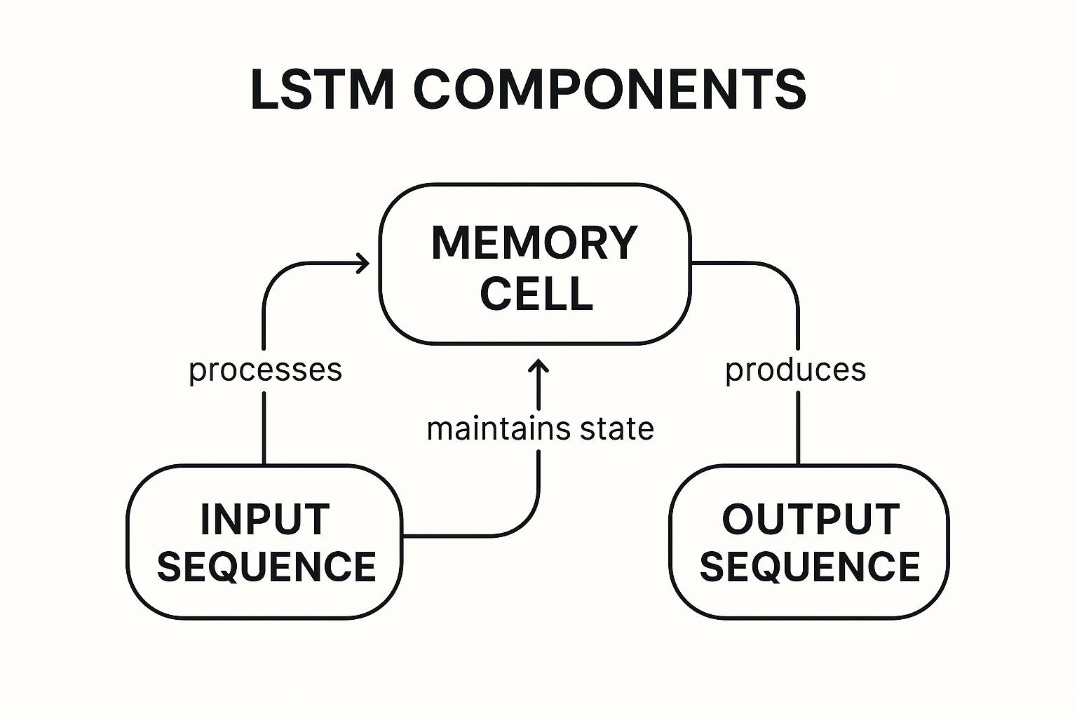
• Flexible sequential representation: LSTMs excel at capturing long-term dependencies, a critical advantage in many time series analysis tasks.
• Handles multivariate inputs naturally: LSTMs can seamlessly process multiple input variables, a common requirement in real-world time series data.
• No stationarity assumptions: Unlike some time series analysis methods, LSTMs do not require the data to be stationary, making them more flexible.
• Effective for both long and short-term dependencies: LSTMs can effectively model both short-term fluctuations and long-term trends in data.

Cons of using LSTMs:

• Data Intensive: Requires a large amount of training data to achieve optimal performance.
• Computationally expensive: Training LSTMs can be time-consuming and resource-intensive, especially with complex architectures.
• Limited Interpretability: LSTMs are often considered "black boxes," making it difficult to understand the underlying reasons behind their predictions.
• Overfitting Risk: Prone to overfitting, particularly with limited data, requiring careful regularization techniques.

Tips for using LSTMs effectively:

• Normalize Input Data: Normalize input data to improve training convergence speed and overall performance.
• Regularization Techniques: Employ dropout and recurrent dropout to mitigate overfitting and improve generalization.
• Start Simple: Begin with simpler LSTM architectures and gradually increase complexity as needed.
• Avoid future leakage: Do not use a bidirectional LSTM for ordinary forward forecasting if its backward direction consumes observations unavailable at prediction time. It is appropriate only when the full input sequence is legitimately available or known future covariates are separated from future targets.
• Multi-step Forecasting: Use sequence-to-sequence architectures for multi-step time series forecasting.

Learn more about Long Short-Term Memory Networks (LSTM) LSTMs were popularized by the groundbreaking work of Sepp Hochreiter and Jürgen Schmidhuber in 1997. Today, frameworks like TensorFlow and PyTorch provide readily accessible tools for implementing LSTMs, and companies like Google and Amazon utilize them extensively for their time series forecasting needs. Their adoption across various industries and their proven ability to handle complex temporal patterns solidify LSTMs as a critical technique in the field of time series analysis.

5. Spectral Analysis

Spectral analysis stands out as a powerful technique within the broader field of time series analysis techniques. It provides a unique lens through which we can understand the underlying cyclical components driving our data. Instead of examining time series data in its familiar sequential form, spectral analysis decomposes it into a sum of sine and cosine waves of different frequencies. This transformation from the time domain to the frequency domain unveils hidden periodicities and oscillatory patterns that might not be readily apparent in standard time-domain plots. This method works by leveraging powerful mathematical tools like the Fourier Transform and Wavelet analysis. The Fourier Transform effectively dissects a time series into its constituent frequencies, revealing the dominant cycles present. Wavelet analysis provides a more nuanced approach, offering better time resolution for analyzing non-stationary time series where frequencies change over time. The output of spectral analysis is often visualized through a periodogram, which displays the power or intensity of each frequency component. The strength of spectral analysis lies in its ability to identify cyclical patterns, even when their periodicity is unknown. This makes it an invaluable tool for exploring complex datasets and uncovering subtle seasonal trends or oscillatory behavior. For example, in macroeconomics, spectral analysis can be used to detect economic cycles by analyzing time series data like GDP or unemployment rates. In neuroscience, it helps decipher brainwave patterns from EEG recordings, identifying characteristic frequencies associated with different cognitive states. Other applications range from analyzing sunspot activity in astronomy to monitoring machinery vibrations for predictive maintenance. Features and Benefits:

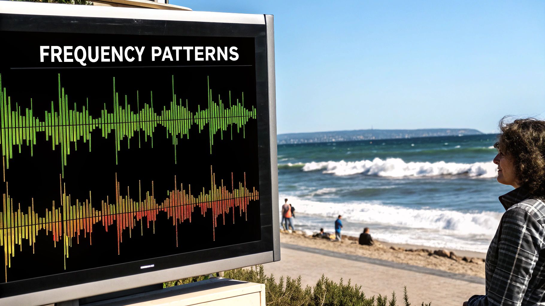
• Transforms data from time domain to frequency domain: Offers a new perspective on data, revealing hidden periodicities.
• Identifies periodic components at different frequencies: Pinpoints the dominant cycles driving the time series.
• Quantifies the strength of cycles and seasonal patterns: Measures the power or intensity of each frequency.
• Can reveal hidden periodicities not obvious in time-domain plots: Uncovers subtle oscillatory behavior.

Pros:

• Effective for identifying cyclical patterns of unknown periodicity: Doesn't require prior knowledge of cycle lengths.
• Useful for noise filtering and signal extraction: Separates signal from noise by isolating specific frequencies.
• Works well for data with multiple overlapping cycles: Can disentangle complex cyclical behavior.
• Provides insights into underlying physical processes: The identified frequencies can relate to underlying mechanisms generating the data.

Cons:

• Assumes stationarity for proper interpretation: Results can be misleading if the time series has trends or changing variance.
• Requires specialized knowledge to interpret results correctly: Understanding of Fourier analysis and signal processing is beneficial.
• Not directly a forecasting method without additional modeling: Further analysis is needed to use the identified cycles for prediction.
• Can be sensitive to irregularly sampled data: Requires pre-processing or specialized techniques for unevenly spaced data points.

Tips for Effective Application:

• Use windowing techniques to reduce spectral leakage: This improves the accuracy of the spectral estimates.
• Consider the tradeoff between frequency resolution and time resolution: Adjust parameters based on the specific characteristics of the data.
• For non-stationary data, consider wavelet analysis instead of Fourier: Wavelets offer better time localization for changing frequencies.
• Use periodogram smoothing to reduce noise in spectral estimates: This enhances the clarity of the dominant frequencies.

Spectral analysis, popularized by the contributions of Joseph Fourier (Fourier Transform), Peter Bloomfield (Fourier Analysis of Time Series), and Ingrid Daubechies (Wavelet Analysis), deserves its place in the list of essential time series analysis techniques. Its unique ability to decompose complex data into its fundamental frequencies provides invaluable insights into cyclical behavior, making it a crucial tool for researchers and practitioners across diverse fields.

6. State Space Models

State space models offer a powerful and flexible approach within the broader field of time series analysis techniques. They provide a unique perspective by representing a time series as a combination of unobserved state variables and observed measurements. This allows for a more nuanced understanding of the underlying dynamics driving the observed data, making them particularly well-suited for complex systems. Instead of directly modeling the observed time series, state space models focus on the hidden states that evolve over time and influence the observed data. This makes them a valuable tool for anyone working with time-dependent data, from data scientists to business executives. How They Work: Imagine an iceberg: you only see the tip above water (the observed data), while a much larger mass remains hidden beneath the surface (the state variables). State space models aim to understand both the visible and hidden parts of the system. They achieve this through two key equations:

• State Equation: This equation describes how the hidden state evolves over time. It incorporates factors like inherent system dynamics, trends, seasonality, and random disturbances.
• Observation Equation: This equation links the hidden state to the observed measurements. It acknowledges that our observations are imperfect and subject to noise.

The Kalman filter, a central algorithm in state space modeling, provides a way to estimate the hidden state based on the noisy observations. This allows us to not only understand the current state but also make predictions about future states and observations. When and Why to Use State Space Models: State space models are particularly valuable in scenarios where:

• Underlying dynamics are complex: They excel at modeling systems with multiple interacting components, such as economic indicators or the movement of a satellite.
• Data is noisy or incomplete: The Kalman filter effectively handles missing observations and separates the underlying signal from noise.
• Real-time analysis is required: The sequential nature of the Kalman filter makes it ideal for updating estimates as new data arrives, enabling dynamic adjustments in applications like GPS navigation.
• Uncertainty quantification is important: State space models provide not only point forecasts but also estimates of the associated uncertainty, which is crucial for informed decision-making.

Features and Benefits:

• Unified framework: State space models provide a single framework that can represent many different time series models, including ARIMA, exponential smoothing, and structural time series models.
• Incorporation of structural components: They can explicitly model trend, seasonality, and cyclical patterns, providing valuable insights into the underlying data generating process.
• Sequential updating: The Kalman filter allows for efficient updates of estimates as new data becomes available, facilitating real-time applications.
• Handling missing data: The Kalman filter naturally handles missing observations without requiring imputation or other ad-hoc solutions.

Pros:

• Handles missing observations elegantly.
• Provides conditionally optimal linear state estimates under a correctly specified linear-Gaussian model.
• Can model complex dynamics in a structured way.
• Well-suited for real-time filtering and smoothing.

Cons:

• Can be mathematically complex to implement from scratch.
• May require strong assumptions about error distributions.
• Parameter estimation can be challenging.
• Computationally intensive for high-dimensional states.

Examples of Successful Implementation:

• Dynamic pricing algorithms in e-commerce: State space models can capture the evolving demand patterns and optimize pricing strategies in real-time.
• GPS navigation systems: They are used to estimate the current location and predict future trajectory based on noisy GPS signals.
• Central banks' economic forecasting: State space models help analyze macroeconomic indicators and predict future economic conditions.
• Target tracking in aerospace and defense: They are crucial for tracking moving objects based on radar or other sensor data.

Tips for Implementation:

• Start with simpler structural models before adding complexity.
• Use maximum likelihood estimation for parameter optimization.
• Consider non-linear extensions (like the Extended Kalman Filter or Unscented Kalman Filter) for complex dynamics.
• Validate model assumptions through residual analysis.

Popularized By:

• Rudolf Kalman (Kalman filter)
• James Durbin and Siem Jan Koopman (Time Series Analysis by State Space Methods)
• Andrew Harvey (structural time series)

State space models deserve their place in the list of essential time series analysis techniques because they provide a powerful and versatile framework for understanding and predicting complex dynamic systems. Their ability to handle noise, incorporate structural components, and provide uncertainty estimates makes them a valuable tool for a wide range of applications, especially when dealing with real-time data and complex underlying dynamics. They empower data scientists, AI researchers, and business executives to extract meaningful insights from time-dependent data and make informed decisions.

7. Vector Autoregression (VAR)

Vector Autoregression (VAR) secures its place among essential time series analysis techniques due to its ability to model multiple interrelated time series simultaneously. Unlike univariate methods that focus on a single time series in isolation, VAR recognizes and quantifies the dynamic interactions between multiple variables, providing a more holistic and realistic representation of complex systems. This makes it a powerful tool for forecasting and analyzing systems where variables influence each other reciprocally. How VAR Works: At its core, VAR extends the principles of autoregression to multiple time series. Each variable's current value is modeled as a linear function of its own past values and the past values of all other variables in the system. This interconnectedness is captured through a system of equations, where each equation represents the evolution of one variable. A VAR coefficient is conditional on the selected variables, transformations, and lag structure; do not interpret one coefficient in isolation as a stable contemporaneous relationship. Use the full dynamic response, uncertainty, residual diagnostics, and identification assumptions where relevant. Features and Benefits:

• Simultaneous Modeling: VAR’s primary strength lies in its ability to model multiple time series concurrently, capturing the intricate web of relationships between them.
• Interdependency Capture: It explicitly models the interdependencies, allowing for a more accurate representation of real-world systems where variables rarely exist in isolation.
• Shock Propagation Analysis: VAR allows for the analysis of how shocks or changes in one variable propagate through the system, affecting other variables over time. This is often done through impulse response analysis.
• Exogenous Variables: The framework is flexible enough to incorporate exogenous variables (variables influenced by factors outside the model) through VARX models.

Pros:

• Comprehensive Analysis: Accounts for the complex relationships between multiple time series, providing a richer understanding compared to univariate methods.
• Predictive precedence: Granger-causality tests ask whether lagged values of one series improve prediction of another within the specified model. They do not establish intervention-level causation; omitted variables, nonstationarity, breaks, and misspecification can change the result.
• Impulse Response Analysis: Enables the study of how shocks to one variable ripple through the system and impact other variables over time.
• Extensible Framework: Can be extended to accommodate cointegrated variables through Vector Error Correction Models (VECM) and structural relationships through Structural VAR (SVAR).

Cons:

• Parameter Proliferation: The number of parameters to estimate grows quadratically with the number of variables, increasing computational complexity and the risk of overfitting.
• Stationarity Requirement: A conventional levels VAR usually requires a stable specification. Transform nonstationary series when appropriate; if series are cointegrated, consider a VECM that preserves the long-run relation. Non-stationary series need to be transformed (e.g., differenced) before using VAR.
• Overparameterization Risk: Can easily become overparameterized, especially with many variables, leading to poor out-of-sample forecasting performance. Careful constraint of parameters is crucial.
• Interpretability Challenges: Interpretation of the model and its coefficients becomes increasingly difficult as the number of variables increases.

Examples of Successful Implementation:

• Macroeconomic Forecasting: Central banks use VAR models to forecast key economic indicators like inflation, GDP growth, and interest rates, taking into account the interdependencies between these variables.
• Financial Market Analysis: Analyzing relationships between related assets (e.g., stocks, bonds, commodities) to understand market dynamics and predict future price movements.
• Energy Market Modeling: Modeling the interplay between different energy sources (electricity, gas, oil) to forecast prices and analyze the impact of policy changes.
• Supply Chain Forecasting: Predicting demand for multiple interdependent products within a supply chain.

Actionable Tips for Effective VAR Modeling:

• Stationarity Testing: Test all time series for stationarity using tests like the Augmented Dickey-Fuller (ADF) test. Difference or transform non-stationary series as needed.
• Lag Selection: Use information criteria like Akaike Information Criterion (AIC) or Bayesian Information Criterion (BIC) to select the optimal number of lags.
• High-Dimensional Data: For high-dimensional data, consider using structured VAR models or Bayesian VAR methods to manage the parameter explosion.
• Cointegration Testing: Test for cointegration between variables. If cointegration exists, a Vector Error Correction Model (VECM) might be more appropriate than a standard VAR.

Popularized By: The development and popularization of VAR models are largely attributed to Christopher Sims, a Nobel laureate in Economics. His work challenged traditional macroeconomic modeling approaches and highlighted the importance of considering interdependencies between variables. Helmut Lütkepohl's book, "New Introduction to Multiple Time Series Analysis," serves as a comprehensive resource on VAR and other multivariate time series techniques. The Federal Reserve and other central banks have adopted VAR models as key tools for macroeconomic forecasting and policy analysis.

8. XGBoost for Time Series

XGBoost (Extreme Gradient Boosting) is a powerful machine learning algorithm widely recognized for its performance in various predictive tasks, and it has proven remarkably adaptable for time series analysis techniques. Unlike traditional time series methods that rely on explicit modeling of temporal dependencies, XGBoost uses a gradient boosting framework to create an ensemble of decision trees. These trees are built sequentially, with each new tree correcting the errors made by its predecessors. This approach allows XGBoost to capture complex non-linear relationships within the data, making it particularly well-suited for time series data exhibiting intricate patterns. For time series applications, the key lies in feature engineering. Instead of directly inputting the time series, relevant features are extracted to represent the temporal dynamics. These features often include lagged values of the time series itself (e.g., the value one hour ago, one day ago, etc.), date-time components (hour of the day, day of the week, month, holidays), and other potentially relevant exogenous variables. By transforming the time series data into a feature-based representation, XGBoost can leverage its powerful tree-based learning algorithm to identify predictive patterns. One of the significant advantages of XGBoost is its ability to incorporate a wide variety of features beyond lagged values. This flexibility makes it particularly useful for scenarios where external factors influence the time series, such as weather data impacting energy consumption or promotional campaigns affecting retail sales. Furthermore, XGBoost handles missing values efficiently and includes built-in regularization techniques to prevent overfitting, enhancing its robustness and generalizability. Features and Benefits:

• Ensemble of gradient-boosted decision trees: Provides high predictive accuracy.
• Feature support requires design: XGBoost can use lagged targets, calendar variables, and external predictors after conversion to supervised rows. Native categorical support requires compatible dtypes and settings; encoding must remain consistent at inference.
• Handles non-linear relationships automatically: Captures complex patterns in time series data.
• Built-in regularization: Reduces overfitting and improves generalization performance.
• Provides feature importance: Offers insights into the drivers of the forecast.

Pros:

• Compare rather than assume: Boosted trees can be competitive when nonlinear relationships and known covariates matter, but no method is universally superior. Compare with seasonal-naive and statistical baselines using rolling-origin evaluation.
• Easily incorporates exogenous variables and categorical features.
• Inspect cautiously: Built-in importance scores describe the fitted model, not causal drivers, and can be unstable or biased by correlated and high-cardinality features.
• Handles missing values efficiently.

Cons:

• Requires careful feature engineering to represent temporal dependencies.
• Less directly interpretable than traditional statistical models (though feature importance helps).
• May struggle with long-term forecasting without proper features.
• Doesn't naturally represent uncertainty in forecasts.

Examples of Successful Implementation:

• Kaggle competition-winning time series forecasts: XGBoost is frequently used in winning solutions for time series competitions.
• Retail demand forecasting with many exogenous factors: Incorporating pricing, promotions, and competitor data.
• Energy consumption prediction incorporating weather variables: Using temperature, humidity, and wind speed as predictors.
• Financial risk modeling: Predicting market volatility and asset prices.

Tips for Using XGBoost for Time Series:

• Create lag features at appropriate intervals: Experiment with different lag periods to capture relevant temporal patterns.
• Include time-based features: Hour of the day, day of the week, month, and holiday indicators can be highly informative.
• Use time-based cross-validation for hyperparameter tuning: Ensure the model generalizes well to future time periods.
• Consider rolling-window approaches for handling concept drift: Adapt to changing patterns in the data over time.
• Combine with statistical methods in ensemble approaches: Leverage the strengths of different methods for improved accuracy.

Learn more about XGBoost for Time Series to explore its implementation using Scala and Spark for big data applications. This resource can provide further insights into handling large-scale time series analysis with XGBoost. XGBoost deserves its place in the list of time series analysis techniques due to its ability to handle complex, non-linear relationships and incorporate a wide range of features. Its strong predictive performance, flexibility, and available tools make it a valuable asset for anyone working with time series data. While it requires careful feature engineering and may not be as interpretable as some traditional methods, its power and versatility often outweigh these limitations, particularly in real-world applications with numerous influencing factors. Popularized by Tianqi Chen and Carlos Guestrin (the original XGBoost developers) and widely adopted by Kaggle competition winners and tech companies like Airbnb and Uber for forecasting, XGBoost has become a go-to method for complex time series problems.

Time Series Techniques Comparison

Method	Useful starting conditions	Key assumptions or risks	Required features/data	Backtest question
Seasonal naive	Stable repeating seasonal pattern	Cannot adapt to changing dynamics	At least one prior season	Does added complexity beat this baseline?
ARIMA/SARIMA	Linear dependence and differencing are adequate	Breaks and misspecification	Ordered univariate history; optional regressors	Are residuals and rolling errors acceptable?
Exponential smoothing	Level, trend, and seasonality dominate	Outliers and structural shifts	Enough cycles for seasonal variants	Are interval coverage and horizon error stable?
Prophet	Several seasons and calendar effects	Trend flexibility and missing daily windows	Future regressors must be known	Does it beat simpler calendar baselines?
LSTM	Enough sequential data and nonlinear signal	Leakage, compute, instability	Chronological windows and available covariates	Does it outperform simpler models out of sample?
State space/Kalman	Latent dynamic-state model is defensible	Distribution and identification assumptions	State and observation equations	Are state uncertainty and forecasts calibrated?
VAR/VECM	Joint dynamics across several series	Lag selection, nonstationarity, identification	Aligned multivariate history	Are forecasts stable across specifications?
XGBoost	Nonlinear lag/covariate effects	Feature leakage and recursive error	Supervised rows with time-safe features	Does rolling evaluation justify complexity?

Mastering Time Series for Data-Driven Success

This exploration of time series analysis techniques, from classical methods like ARIMA and Exponential Smoothing to cutting-edge approaches like LSTM networks and XGBoost, has provided a solid foundation for making data-driven decisions. Whether you're forecasting market trends, optimizing supply chains, predicting equipment failure, or understanding customer behavior, these methods empower you to extract valuable insights from your temporal data. We've covered a range of techniques including Spectral Analysis, State Space Models, and Vector Autoregression (VAR), each offering unique strengths for different types of time series data. For businesses focused on customer retention, accurately forecasting churn is paramount. Leveraging time series analysis in conjunction with a customer health score can provide powerful predictive capabilities and inform targeted interventions. The key takeaway is that choosing the right time series analysis techniques depends heavily on the specific characteristics of your data and the problem you're aiming to solve. Experimentation, continuous learning, and a deep understanding of the underlying principles are crucial for success. Mastering these concepts allows you to not only analyze past trends but also to anticipate future events, mitigate risks, and ultimately, gain a competitive edge in today’s data-driven world. Ready to elevate your time series analysis capabilities? Data4AI provides advanced tools and resources, including pre-built models and automated workflows, to simplify and accelerate your time series projects. Visit Data4AI archive today to discover how you can unlock the full potential of your time-based data and drive impactful decisions.