Build a CNN with Keras: Step-by-Step Tutorial

Convolutional neural networks (CNNs) remain a foundational architecture for image classification and many other vision tasks. They are no longer the only dominant approach—vision transformers and hybrid architectures are also widely used—but CNNs are still an excellent way to learn spatial feature extraction and build an efficient baseline.

Instead of just looking at a flat list of numbers, a CNN learns to recognize features in an image, building up its understanding from simple edges all the way to complex objects. This guide will provide actionable insights and practical examples to get you started.

How a CNN Actually Learns to See

Before we jump into any code, it’s really important to get a gut feeling for what a CNN is doing under the hood. Unlike a standard neural network that flattens an image into a long vector of pixels, a CNN is designed from the ground up to respect the spatial structure of an image. It doesn't see a "cat" right away. First, it sees the basic building blocks—edges, textures, shapes, and patterns—that, when pieced together, form the concept of a cat.

CNNs use local connectivity and shared weights to exploit spatial structure. Their development drew some historical inspiration from research on biological vision, but modern CNNs should not be described as literal models of the visual cortex. LeNet-5, published by Yann LeCun and collaborators in 1998, demonstrated gradient-based recognition of handwritten document images and became an important milestone.

The Building Blocks of a CNN

A CNN is essentially a stack of specialized layers, and each layer has a very specific job to do. If you're just getting started, you might want to check out our guide on neural network basics to get your bearings first. Once you understand what each layer does, building and troubleshooting your own models becomes much more intuitive.

Here are the three main players you'll be working with:

• Convolutional Layers: These are the heart and soul of the network. They use filters (also called kernels) that slide across the input image to hunt for specific features. Early on, these filters might pick up on simple things like vertical lines or color gradients. As you go deeper into the network, the layers learn to combine these simple features into more complex patterns, like an eye or a car's wheel.
• Pooling Layers: Right after a convolutional layer has done its job extracting features, a pooling layer comes in to clean things up. It shrinks the spatial size of the data, usually through a process called max pooling. This makes the network more efficient and helps it focus only on the most significant features that were detected.
• Fully Connected Layers: These sit at the very end of the network. They take all the high-level features extracted by the previous layers and do the final classification. Think of them as the decision-makers that look at the evidence and make the final call, like labeling an image as a "dog" or a "cat."

To make this clearer, here's a quick breakdown of what each layer is responsible for.

Key CNN Layers and Their Functions

Layer Type	Primary Function	Key Analogy
Convolutional	Feature Detection	A detective using different magnifying glasses (filters) to find specific clues (features) like fingerprints or footprints in an image.
Pooling	Downsampling & Dimensionality Reduction	Summarizing a long book into a one-page synopsis. It keeps the most important information while making it much smaller and easier to handle.
Fully Connected	Classification & Decision-Making	The final jury that takes all the evidence presented by the detectives and decides on a verdict ("cat" or "dog").

By stacking these layers, a CNN creates a powerful feature hierarchy. It starts with the tiny details and gradually builds up a more abstract, complete understanding of what's in the image.

The real power of a CNN is that it learns what features to look for on its own. We don't have to manually program it to find edges or textures; it figures out the best filters during the training process.

This automated feature learning is precisely what makes CNNs so incredibly effective for image-related tasks. In the rest of this tutorial, we'll get our hands dirty and actually build each of these layers from scratch.

Getting Your Python Environment Ready for Deep Learning

This tutorial uses the current standalone Keras API with TensorFlow as the backend. Create an isolated virtual environment and check the current TensorFlow installation guide for your operating system before installing, because GPU support differs across Linux, WSL2, native Windows, and macOS.

python3 -m venv .venv
source .venv/bin/activate  # Windows PowerShell: .venv\Scripts\Activate.ps1
python -m pip install --upgrade pip
python -m pip install tensorflow notebook

On supported Linux or WSL2 systems with an NVIDIA GPU, TensorFlow documents a separate tensorflow[and-cuda] installation path. Current official TensorFlow packages do not provide native macOS GPU support, and native-Windows GPU support ended after TensorFlow 2.10. Do not assume that a generic pip install tensorflow enables GPU acceleration on every platform.

import tensorflow as tf
import keras

print("TensorFlow:", tf.__version__)
print("Keras:", keras.__version__)
print("Visible GPUs:", tf.config.list_physical_devices("GPU"))

A GPU can accelerate training, but the speedup is workload- and hardware-dependent. This small CIFAR-10 model can be completed on a CPU; avoid promising a universal 10×–50× improvement.

Record your Python and package versions with the experiment. Reproducibility is more useful than an environment that merely worked once.

Building a CNN for Image Classification From Scratch

Alright, we've covered the theory and have our environment ready to go. Now it's time to roll up our sleeves and actually build something. This is where we bridge the gap between abstract concepts and real, working code. We're going to build a functional image classifier from the ground up using Keras, a wonderfully intuitive API that lives inside TensorFlow. You'll be surprised how straightforward it is to construct a fairly complex network.

Our model's first challenge will be the CIFAR-10 dataset, a classic benchmark in the computer vision world. It’s a collection of 60,000 tiny 32x32 color images spread across ten distinct classes—think 'airplane', 'automobile', 'bird', and 'cat'. Our mission, should we choose to accept it, is to train a CNN that can correctly identify what's in a new image from this dataset.

Loading and Preparing the Data

Keras provides CIFAR-10 as 50,000 training images and 10,000 test images. Each image is 32×32 pixels with three color channels, and each label is an integer from 0 through 9. Scale the pixel values to the 0–1 range and keep the integer labels so the model can use sparse categorical cross-entropy.

import keras

(x_train, y_train), (x_test, y_test) = keras.datasets.cifar10.load_data()
x_train = x_train.astype("float32") / 255.0
x_test = x_test.astype("float32") / 255.0
y_train = y_train.reshape(-1)
y_test = y_test.reshape(-1)

num_classes = 10
input_shape = (32, 32, 3)

The test split must remain untouched during model selection. We will reserve part of the training data for validation during fit() and evaluate on x_test only after training decisions are complete.

Designing the CNN Architecture

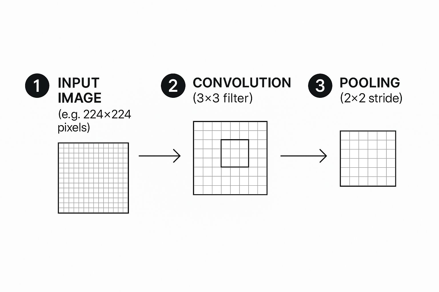
Now for the fun part: actually designing the model layer by layer. A standard CNN for image classification begins with a series of convolutional and pooling layers to find patterns, then flattens that information to feed into dense layers that make the final call.

This infographic gives a great visual overview of how an image gets processed through convolution and pooling, which are the foundational blocks of our network.

This cycle of feature extraction and downsampling is what allows the network to build a hierarchy of features, starting with simple lines and colors and building up to more complex shapes and objects.

Our model will follow this proven blueprint. We'll stack a few Conv2D layers, each followed by a MaxPooling2D layer. The early convolutional layers will be on the lookout for basic features like edges and gradients. As data flows deeper, later layers will combine these simple patterns to recognize more intricate things like textures or parts of an object.

The number of filters in a convolutional layer is a key hyperparameter to tweak. A common and effective strategy is to start with a smaller number, like 32, and increase it in deeper layers. This lets the network learn a wider variety of more abstract features as it goes.

After the feature extraction stage, a Flatten layer converts the 2D feature maps into a long, 1D vector. This vector is then passed to one or more Dense (or fully connected) layers, which handle the final classification logic.

The very last layer is a Dense layer with a neuron count equal to our number of classes—10 in this case—and a softmax activation function. Softmax is perfect for this job because it converts the network's raw output scores into a set of probabilities that sum to one, giving us a clear prediction for each class. Getting a handle on how different activation functions work is really important; our guide on neural network activation functions dives much deeper into this topic.

The Complete Model

The current Keras pattern starts a Sequential model with an explicit keras.Input. This compact baseline adds dropout before the classifier; it is intentionally educational rather than state of the art.

from keras import layers

model = keras.Sequential([
    keras.Input(shape=input_shape),
    layers.Conv2D(32, 3, padding="same", activation="relu"),
    layers.MaxPooling2D(),
    layers.Conv2D(64, 3, padding="same", activation="relu"),
    layers.MaxPooling2D(),
    layers.Conv2D(128, 3, padding="same", activation="relu"),
    layers.MaxPooling2D(),
    layers.Flatten(),
    layers.Dense(256, activation="relu"),
    layers.Dropout(0.4),
    layers.Dense(num_classes, activation="softmax"),
])

model.summary()

model.summary() reports tensor shapes and parameter counts and is a useful architecture sanity check.

Getting Your CNN Ready to Train and Evaluate

So far, all we have is a blueprint. Our CNN architecture is defined, but it's an empty shell with no real knowledge. The next step is where the magic happens: we're going to breathe life into it through training.

This is the part where we teach the network how to tell images apart by showing it thousands of examples. We'll start by setting up its learning strategy and then kick off the process of feeding it data.

Compiling and Training Without Test Leakage

Compile the model with Adam and sparse categorical cross-entropy because the labels remain integer encoded. Accuracy is useful for this balanced introductory dataset, but production evaluation may require per-class metrics, calibration, robustness tests, and error analysis.

model.compile(
    optimizer="adam",
    loss="sparse_categorical_crossentropy",
    metrics=["accuracy"],
)

early_stopping = keras.callbacks.EarlyStopping(
    monitor="val_loss",
    patience=3,
    restore_best_weights=True,
)

history = model.fit(
    x_train,
    y_train,
    batch_size=64,
    epochs=30,
    validation_split=0.1,
    callbacks=[early_stopping],
)

The final 10% of the training arrays becomes the validation split in this simple example. For reproducible research or class-imbalanced data, create an explicit shuffled or stratified split instead. The separate test set is not supplied to fit().

Making Sense of the Training Logs

As .fit() runs, you'll see a stream of logs flooding your screen for each epoch. It might look like a jumble of numbers at first, but this output is pure gold.

Each line gives you a snapshot of the training progress:

• loss: The training loss for the current epoch. You want this to go down, down, down.
• accuracy: The training accuracy. This should steadily climb upwards.
• val_loss: The validation loss (calculated on the test set). This is the one to watch. If it starts creeping up while the training loss is still falling, your model is probably overfitting.
• val_accuracy: The validation accuracy. This is your most honest measure of how the model is performing on data it hasn't seen before.

Pro Tip: Keep a close eye on val_loss. The moment it flattens out or starts to rise is often the perfect time to stop training. This technique, called early stopping, is a simple but powerful way to build more robust models that don't just memorize the training data.

Evaluating the Final Model Performance

Once the training is done, it's time for the final report card. We need an unbiased assessment of our model's true capabilities. For this, we use the .evaluate() method on our test dataset—data the model has never used to adjust its weights.

This gives us the definitive measure of its performance.

test_loss, test_accuracy = model.evaluate(x_test, y_test, verbose=2)
print(f"Test accuracy: {test_accuracy:.4f}")

The output reports loss and accuracy on the held-out CIFAR-10 test set. Results vary with software versions, hardware, random initialization, preprocessing, and training choices, so this tutorial does not promise an accuracy range. CIFAR-10 performance is evidence about this benchmark—not a guarantee of performance on real-world images from a different distribution.

Actionable Techniques to Improve Model Accuracy

Getting your first convolutional neural network to run is a huge win. Seeing it achieve a decent baseline accuracy? Even better. But that's where the real work begins. The gap between a basic model and a high-performing, production-ready one is closed by applying a few key refinement techniques.

Most of these techniques are designed to fight one of the biggest enemies in deep learning: overfitting.

Overfitting is what happens when your model gets a little too good at its job. It memorizes the training data—including all its noise and quirks—but then falls flat when it sees new, real-world images. You can spot it when your training accuracy keeps climbing, but your validation accuracy stalls out or even starts to dip.

Let's walk through some practical, battle-tested strategies to combat this and really boost your model's performance.

Use Training-Time Data Augmentation Carefully

Data augmentation creates plausible variations of training examples. The transformations must preserve the label: horizontal flips may be reasonable for CIFAR-10, while flips or rotations can be wrong for text, medical orientation, or direction-sensitive classes. Current Keras preprocessing layers apply augmentation during training and are inactive during evaluation.

data_augmentation = keras.Sequential([
    layers.RandomFlip("horizontal"),
    layers.RandomRotation(0.05),
    layers.RandomTranslation(0.1, 0.1),
])

# Place this immediately after keras.Input(...) in the model:
# data_augmentation,

Compare an augmented run against the same baseline and validation protocol. Augmentation often helps when its invariances match the problem, but it is not guaranteed to improve every dataset.

Build Resilience with Dropout Layers

Another incredibly powerful tool in your anti-overfitting toolbox is dropout. The concept behind it is brilliantly simple: during each step of the training process, you randomly "drop" or temporarily disable a fraction of the neurons in a layer.

This forces the remaining active neurons to learn more robust and independent features because they can't afford to rely on any single neuron always being there.

Think of it like training a basketball team where you randomly bench a few players during every practice drill. The team quickly learns how to play together without becoming overly dependent on any one star player.

This makes the entire network far less sensitive to the specific weights of individual neurons, which is a classic symptom of overfitting. Adding a Dropout layer is a one-line change in Keras that can have a massive impact.

Dropout rate is a tunable hyperparameter, not a universal prescription. Values such as 0.2–0.5 are commonly explored, but the appropriate rate and placement should be selected with validation data.

from tensorflow.keras.layers import Dropout

model.add(Flatten())
model.add(Dense(512, activation='relu'))
model.add(Dropout(0.5)) # Deactivates 50% of neurons in the previous layer
model.add(Dense(num_classes, activation='softmax'))

For a deeper dive, check out our guide on how to effectively use dropout in a neural network to prevent these kinds of complex co-dependencies from forming.

Overfitting is a common challenge, but data augmentation and dropout are just two of several effective solutions. Here's a quick comparison of some simple yet powerful techniques you can use.

Common Overfitting Solutions

Technique	How It Works	When to Use It
Data Augmentation	Creates modified versions of existing training data (e.g., rotations, flips).	Almost always a good idea, especially with limited image datasets. It's a low-cost way to expand your training set.
Dropout	Randomly deactivates a fraction of neurons during training to prevent co-dependency.	Excellent for dense layers in your network, but can also be used after convolutional layers. A go-to regularizer.
Early Stopping	Monitors validation loss and stops training when it no longer improves.	A simple and effective way to prevent the model from training for too long and memorizing the training data.
L1/L2 Regularization	Adds a penalty to the loss function based on the magnitude of the layer weights.	Useful when you suspect many features are irrelevant (L1) or want to prevent weights from becoming too large (L2).

Each of these methods tackles the problem from a slightly different angle, and they can even be used together to create a more resilient and generalizable model.

Fine-Tuning Hyperparameters for Better Results

Finally, never be afraid to roll up your sleeves and experiment with your model's hyperparameters. These are the settings you define before training starts, and they can dramatically influence your final accuracy. There’s no magic formula here, but systematically tweaking them can unlock significant performance gains.

Here are a few of the most important ones to focus on:

• Learning Rate: This is probably the most critical hyperparameter. If it’s too high, your optimizer might leap right over the best solution. Too low, and training will take forever. Start by adjusting the default in your optimizer (e.g., Adam(learning_rate=0.0001)).
• Number of Filters: The number of filters in your Conv2D layers (32, 64, 128, etc.) controls how many features the model can learn at each level. If your model is underperforming, try gradually increasing the filter count to give it more capacity.
• Batch Size: This determines how many samples are processed before the model's weights are updated. Smaller batch sizes can introduce a bit of helpful noise, while larger ones provide a more stable gradient. Experiment with powers of two like 32, 64, or 128 to see what works for your dataset.

By methodically applying these techniques—data augmentation, dropout, and hyperparameter tuning—you'll move beyond just building a basic CNN and start engineering a truly high-performing model.

Common Questions About Building CNNs

As you start piecing together your own convolutional neural networks, you're bound to run into some questions. It's totally normal. Building these models has a lot of moving parts, and hitting a roadblock is just part of the learning curve. Let's walk through some of the most common hurdles I've seen and get you some clear, actionable answers.

Dense vs. Convolutional Layers

So, what's the deal with dense and convolutional layers? What's the real difference?

Think of them as specialists with completely different jobs. A convolutional layer is your feature detective. Its whole purpose is to scan an image with filters to pick out spatial patterns—things like edges, specific textures, or even basic shapes. It's all about finding those localized features.

A dense layer (you'll also hear it called a fully connected layer) usually comes in at the end of the network. It takes all the high-level features that the convolutional layers have found and does the final classification work. Every neuron in a dense layer is connected to every single neuron from the layer before it, which lets it learn the non-spatial patterns from all the combined features. This is where the final decision gets made, like labeling an image as "cat" or "dog."

Why Model Accuracy Stagnates

It’s incredibly frustrating when you're training a model and the accuracy just stops improving. This is a classic problem known as a performance plateau, and it usually points to one of a few common culprits.

First, check your learning rate. If it’s too high, your optimizer is probably overshooting the best solution every time it updates. If it's too low, it's learning so slowly that it can't make any meaningful progress in a reasonable amount of time.

Another real possibility is that your model's architecture is just too simple for how complex your dataset is. A shallow network might not have enough capacity to learn the really intricate patterns hidden in the data.

Actionable Tip: Before you go tearing your model apart, try systematically adjusting the learning rate. A little tweak here can make a big difference. If that doesn't move the needle, then consider adding another convolutional block or implementing data augmentation to give your model more varied examples to learn from.

Determining the Right Number of Epochs

How many epochs should you train for? There’s no magic number here. The ideal amount depends entirely on your specific model and dataset.

Train for too few epochs, and you end up with underfitting—the model just hasn't had enough time to learn from the data. But if you train for too many, you risk overfitting, where the model starts memorizing the training data instead of learning how to generalize to new, unseen data. Our article on epochs in machine learning covers this trade-off in more detail.

The best practice is to keep a close eye on your validation loss, not just the training accuracy. When that validation loss stops decreasing and either flattens out or starts to creep back up, that’s your cue to stop training. You've hit the point of diminishing returns, which is often the sweet spot for getting the best performance.

CNNs remain useful components and baselines, but modern computer-vision systems may also use transformers, hybrid architectures, pretrained backbones, or task-specific models. Choose an architecture through representative evaluation rather than assuming one family is universally best.

Primary references

1. Keras 3: CIFAR-10 dataset
2. Keras 3: simple convolutional network example
3. Keras 3: image classification and augmentation
4. TensorFlow: current pip installation and platform support
5. LeCun et al. (1998): Gradient-Based Learning Applied to Document Recognition

Fact-check record

Reviewed September 4, 2026. The tutorial was updated for current Keras conventions. The test-set leakage was removed, installation and GPU claims were corrected by platform, obsolete augmentation code was replaced with Keras preprocessing layers, benchmark-performance promises were removed, and CNNs were positioned alongside—not above—modern vision alternatives.

---